X and the City: Modeling Aspects of Urban Life (36 page)

(iii)
bT
= 1; both roots are pure imaginary, and the solution is oscillatory (neutrally stable).

(iv)
bT
> 1; both roots are complex, and the solution is increasing and oscillatory (unstable).

What does all this mean? Remember that the solution
u
_n
(
t
) =
Ue
^pt
is the speed of the
n
th vehicle in the line of traffic. From cases (i)–(iv) we see that (locally at least) the speed can decrease, oscillate about a decreasing mean value, oscillate about a constant mean value, and oscillate about an increasing mean value. This last case is indicative of the potential for collisions somewhere down the traffic line. The model is a crude one, to be sure, but this latter behavior is also consistent with the solution for the nonhomogeneous equation, known as the “particular integral.” The choice of functional form sought depends on that of the presumed known quantity
u
_n
−1
(
t
), but for our purposes
it is sufficient, in light of (i)–(iv) above to consider an oscillatory solution of the form
. Substituting this in equation (12.10) results in the expression

Note that

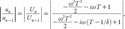
and this ratio grows as
n
increases if the expression on the right exceeds unity. Note that this term can be written in simplified form in terms of real and imaginary parts as

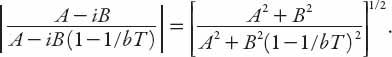
It is clear that we require
bT
> 1/2 for |
u
_n
/
u
_n
−1
| > 1. This then supersedes the previous criterion for instability because it “kicks in” at a lower value of
bT
.

For completeness in this section, the exact solution for this problem is stated below:

(i) 0 ≤
bT
≤
e
⁻¹
≈ 0.368; both roots are negative and the solution is exponentially decreasing (stable).

 (ii)
e
⁻¹
<
bT
<
π
/2 ≈ 1.571; both roots are complex, and the solution is damped oscillatory (stable).

(iii)
bT
=
π
/2; both roots are pure imaginary, and the solution is oscillatory (neutrally stable).

(iii)
bT
>
π
/2; both roots are complex, and the solution is increasing and oscillatory (unstable).

The rough and ready calculations therefore have the right “character traits” insofar as stability and instability are concerned, but the transition points are
inaccurate. However, it must be said that compared with the exact solution, the upper bound in part (i) above is an overestimate of only 11%, while the transition value in part (iii) is an underestimate of about 36%.

Exercise:
Show that, had we expanded equation (12.9) as a linear Taylor polynomial in
T
only, the results would have been very similar:

for the homogeneous solution and

What percentage of our (waking) time do we spend driving? In the United States, a typical drive to and from work may be at least half an hour each way, frequently more in high density metropolitan areas. So for an 8-hr working day, the drive adds at least 12–13% to that time, during much of which drivers may become extremely frustrated. (Confession: I am not one of those people; I am fortunate enough to walk to work!)

On 25 January 2011 my local newspaper carried an article entitled “Slow Motion.” The article took data from the American Community Survey (conducted by the U.S. Census Bureau) and presented average commuter travel times for the region. According to the survey, the NYC metro area had the highest “average commute time,” more than 38 minutes; Washington, DC, was
second with 37 minutes, and Chicago was third with more than 34 minutes. (The piece in the newspaper stated the commute times to the nearest hundredth of a minute—about half a second—which is clearly silly!) The average for my locality was about 26 minutes.

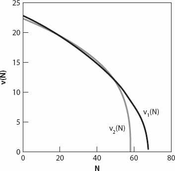
In much of what follows, the equations describing various features of traffic-related phenomena are based on detailed observational studies published in the literature. Consequently, the coefficients in many of these equations are not particularly “nice,” that is, not integers! For example, one measure of the capacity of a road network in a UK city center (London) was given by [
25
]

where
v
₁
is the average speed of traffic in mph (numerically). The traffic flow is more easily appreciated by inverting this to give the approximate expression
v
₁
= (523 − 7.7
N
)
^1/2
. For comparison, another empirical measure is also illustrated:

As can be seen from
Figure 13.1
, the two formulae give similar results for speeds above about 12 mph, but in fact
v
₁
(
N
) (solid curve) is a better fit to the low-speed data. It should be emphasized that both
N
and
v
_1,2
are numerical values associated with the units in which they are expressed, so equation (13.1) and others like it are dimensionless.