X and the City: Modeling Aspects of Urban Life (38 page)

Therefore, if
N
is the flow before I try to sneak my car into the traffic, the total increase in journey time of the other vehicles is approximately
Nδt
/
δN
, that is, −
Nlv
′(
N
)/
v
²
. I do feel a little guilty about this, but I have to get to the bank before it closes. Using equation (13.2) this can be rewritten as

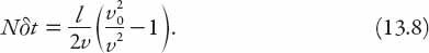
We can extract more from this equation. The journey takes a time
l/v
, so that

As may be seen from equation (13.9), this represents a significant time loss if the speed of traffic is low. And here is another point to note: equation (13.8) represents the time loss imposed on other vehicles by my entry into the traffic stream. If we add to this the time loss sustained by my vehicle, then the resulting sum must be the same as that expressed by equation (13.5), that is,

Exercise:
Verify this identity.

X
=
dx
/
dt
: Question:
How fast do traffic back-ups increase in length?

As we all know from experience, delays while driving can arise for several reasons: accidents or other obstructions, tunnels, bottlenecks at an intersection, raised bridges, or even a poorly adjusted traffic light at a busy junction. If the traffic flow is
N
vehicles at speed
v
, and joins a line of traffic (a traffic queue if you are reading this in the UK) with average flow
N
₀
at speed
v
₀
, no line forms if
N
<
N
₀
. By contrast, if
N
>
N
₀
, a steadily increasing line forms (we are here excluding temporary back-ups that oscillate in length). In the latter case, the rate at which the line lengthens can be computed as follows. We denote the length of the back-up be
x
at time
t
, where
x
(0) = 0, that is, we suppose that the problem starts at time “zero.” Noting that the ratio
N/v
has units of (vehicles/hr) ÷ (mph), or vehicles/mile, it follows that at
t
= 0, a portion of road of length
x
contains
Nx
/
v
vehicles. At a later time
t
it contains
N
₀
x
/
v
₀
, because of the back-up. Therefore the number of vehicles entering the stretch minus the number leaving it is (
N
−
N
₀
)
t
, but this is just the quantity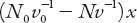
. Hence the rate at which the back-up increases is

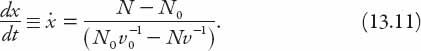
In the question below we apply this formula to an all-too-common situation in many parts of the world.

Question:
Suppose the traffic is stationary. How fast is the line of traffic increasing?

This means that
N
₀
= 0 and
v
₀
= 0; clearly this means that equation (13.11) is indeterminate, so how are we to interpret the ratio
N
₀
/
v
₀
in this case? Dimensionally,
N/v
is the ratio of vehicles per unit time to speed, that is, vehicles/length, or vehicular density on the road. In the case of stationary traffic, as here, this is just the concentration of vehicles in the queue. We shall take the
effective length
of an “average” vehicle to include the space between each one and the vehicle ahead. As before, we’ll call this density
k
, so equation (13.11) reduces to

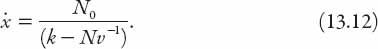
This is the rate at which the traffic “jam” lengthens. Suppose, as an example, that we take the effective length for American vehicles (including the gap ahead) to be about 25 ft (it is probably less in Europe since the cars are typically smaller), and that the vehicles arrive at 30 mph, with a flow rate of, say, 500 vehicles per hour. The concentration per mile of the stationary line of cars,
k
, is then 5280 ÷ 25 ≈ 210 per mile. From (13.12) the line increases at a rate

Obviously, one can plug in one’s own estimates based on different traffic conditions.

X
=
: Question:
What is the average distance traveled in a city/town center?

This can be quite a complicated quantity to calculate, depending as it does on the type of road network and distribution of starting points and destinations, among other factors. Smeed (1968) assumed a uniform distribution of origins and destinations for both idealized and real UK road networks, and with some simplifying assumptions, concluded that the range of values lay between 0.70
A
^1/2
and 1.07
A
^1/2
, with a mean of 0.87
A
^1/2
,
A
being the area of the town center (assuming this can be suitably defined). Obviously the factor
A
^1/2
renders the result dimensionally correct. With this behind us, the next stage is to try to determine the average length of a journey during say, a peak travel period. Using rather sophisticated statistical tools, Smeed was able to calculate the above average distance traveled on roads of any given town or city center,
assuming only that the journeys are made by the shortest possible route. Rather than try to reproduce the (unpublished) calculations here, let us try to make these figures plausible on the basis of some simple geometric models of cities.