X and the City: Modeling Aspects of Urban Life (31 page)

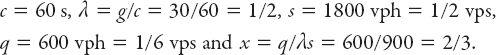
Then

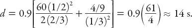
Webster also derived two expressions for the average length
L
of a traffic line (or queue) at the beginning of a green phase (usually the maximum length in the cycle). The first and least accurate one is

where the new parameter
r
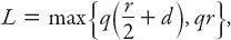
is the “red time.” This underestimates the length by 5–10% because it is based on the assumption that vehicles do not join the line until they have reached the stop line. A more accurate formula incorporating three new parameters is

that is, each term is increased by the factor
, where
y
is the average spacing between vehicles in the line,
a
is the number of lanes and
v
is the “free running speed” of the traffic.

How does the fundamental diagram “square” with known traffic configurations in tunnels (where the likelihood of traffic jams is quite high, especially during rush hour)? The Lincoln Tunnel (under the Hudson River) in New York City has a maximum traffic flow of about 1600 vph (vehicles per hour) at a density of about 82 vehicles per mile moving at a mean speed of 19 mph (see
Table 10.1
and the scatter plot in
Figure 10.2
). As noted, if the density is almost zero, the traffic flows at the maximum speed, and for a range of small densities remains nearly constant, so the flow varies almost linearly with density in this range,
q
≈
ku
_max
. This is consistent with measurements in both the Lincoln Tunnel and other NYC tunnels such as the Holland and Queens Midtown Tunnels. As the density increases, with a corresponding increase in flow, these same measurements show differences in the
q-k
curves: both the capacity and the corresponding speed are lower in the older tunnels (Haberman 1977). This should not be too surprising given that newer tunnels typically have greater lane width and improved lighting that permit higher speeds at the same traffic concentrations. Furthermore, the capacity of a given tunnel may vary along the road—regions with lower capacity than elsewhere are called bottlenecks, and in tunnels they typically occur on the “upward and outward” part of the tunnel (why do you think this is?).

T
ABLE
10.1

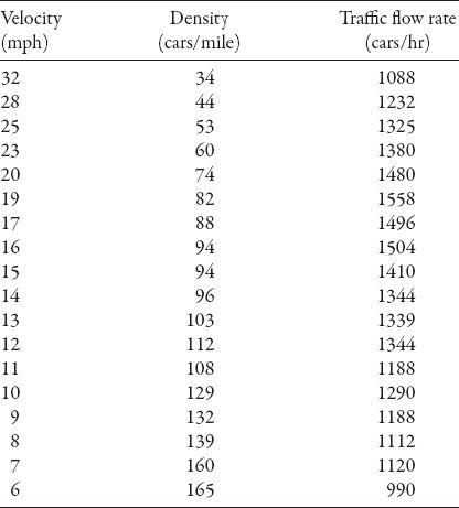
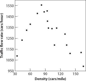
Figure 10.2. Scatter plot of data from
Table 10.1
.

Ideally, traffic should be forced somehow to maintain maximum flow by manipulating the density and speed appropriately. In my (limited) experience this works well on the M25 “orbital” motorway around London, which has variable speed limits (and speed cameras) during rush hour. In the Holland Tunnel, momentarily stopping traffic resulted in increased flow! This is because a traffic signal at the entrance to the tunnel was suitably timed to permit traffic to flow in intervals with density corresponding to the maximum flow.

Don’t some cars inevitably follow others, and not just in the city? They certainly do, but the phrase as used here means that we model traffic by identifying each car as a separate object, not just part of the flow of a fluid called “traffic.” We’ll start by setting up a particular type of differential equation for this (now) discrete system.

Suppose that the position of the
n
th car on the road is
x
_n
(
t
). If we disallow passing in this model we can assume that the motion of any car depends only
on that of the car ahead. A simple approach is to set the car’s acceleration proportional to the relative speed between it and the car in front; thus we have

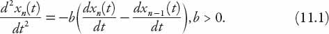
This means that if the
n
th car is traveling faster than the one in front, it must decelerate to avoid a collision (generally a good idea). Conversely, if it is not traveling as fast as the one in front, the driver will (in this model) accelerate accordingly. Note that the model, simplistic as it is, does not give the driver the choice of maintaining a constant speed unless the right-hand side of equation (11.1) is zero. Additionally, the equation takes no account of the time lag due to the reaction time (
T
) of the driver in responding to the changing conditions ahead of her.

(At this point the reader may throw up his hands in disgust and say—“These mathematicians! Nothing is ever realistic—when do such conditions
ever
occur?” He has my sympathies, but this is the way modeling is usually done: take the simplest nontrivial situation and see what the implications are for the real-world problem, and modify, tweak, and improve as necessary . . . trial and error are important in constructing models.)

Incorporating the reaction time
T
results in the modification