X and the City: Modeling Aspects of Urban Life (45 page)

Hence the number of person-years lived is, from (15.16),

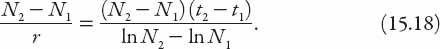
The left-hand side, expressed in person-years, can be converted to persons by dividing by a time factor. This should be an average life expectancy, but that is very difficult to determine, even if known in principle, owing to gender,
regional, and temporal variations. For example, extracting possibly relevant (i.e., Northern European) data from a table in the
Encyclopedia Britannica
(1961), we have:

In view of these “data” we shall take an average of
r
⁻¹
= 40 years for the range 1801–2006 considered in
Table 15.1
, and estimate the quantity

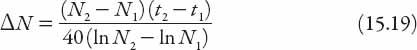
T
ABLE
15.1

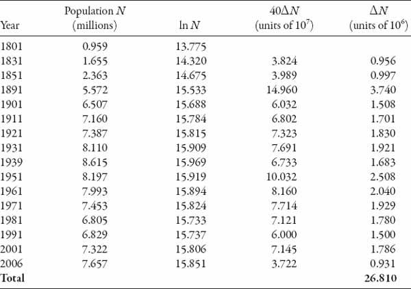
for a range of data points. Summing all these from the table we have the estimate of

Clearly this is a rough-and-ready approach, dependent on the width of the time intervals and the reliability of the data. The result is not particularly sensitive to the choice of life expectancy, but it
is
sensitive to the number of intervals chosen in the overall time frame. The more intervals we choose, assuming the data are available, the more different the cumulative population will generally be. To see this, just take a
single interval
from 1801 to 2006. We take
t
₁
= 1801 and
t
₂
= 2006, and
N
₁
= 9.59 × 10
⁵
,
N
₂
= 7.66 × 10
⁶
. Using equation (15.19), we find that
N
_tot
(now equal to Δ
N
of course) ≈ 16.7 million. If we were to go back to the years
t
₁
= 1000 and
t
₂
= 2600 as before, then
N
₁
≈ 10
⁴
and
N
₂
is again as before. The corresponding value of
N
_tot
is now 290 million for the same value of
r
. Obviously the value for London’s population in the year 1000 is somewhat suspect, but this is just to illustrate the point regarding the interval width. The average lifetime was probably lower in medieval times, so if we set
r
⁻¹
= 30 yr then
N
_tot
increases to 386 million.

Nevertheless, this is an interesting application of some simple mathematics, and is probably far more reliable than estimates of all the people who have ever lived (Keyfitz 1976)!

In light of the above comments, it is somewhat surprising that fairly general quantitative patterns of urban population density
ρ
(population per unit area) can nevertheless be formulated for single-center cities. As far back as 1951 Colin Clark, a statistician, compiled such data for 20 cities, and found that
ρ
declined approximately exponentially with distance from city centers (though “city center” is not always easily defined in practice;
central business district
is perhaps a better term). If we restrict ourselves to the special but important case of circular symmetry, wherein
ρ
=
ρ
(
r
),
r
being the radial coordinate, then naturally we expect that
ρ
′(
r
) < 0, but also perhaps that the density drops off more gradually as
r
increases, that is,
ρ
″(
r
) > 0. Furthermore, we might anticipate that this density profile gets flatter
as the “boundary” of the city is approached. If we consider the simplest possible model of exponential decline, the suggested conditions for
ρ
are satisfied, so let us consider

A
and
b
being positive constants; in fact from (16.1),
A
=
ρ
(0) ≡
ρ
₀
and
b
= −
ρ
′(0)/
ρ
₀
. Of course, in practice, urban population growth is a dynamic process, so to be more general we should permit
A
and
b
to be time-dependent (and this we shall do shortly). In fact, several values of
A
and
b
reported for London over a period of 150 years are listed below, along with correspondingly less information for three other cities, Paris, Chicago, and New York. Before analyzing these data, we derive an expression for the population.

The total metropolitan population in a disk of radius
R
₀
is given by the integral