X and the City: Modeling Aspects of Urban Life (42 page)

where
C
is a constant of integration. This can be found immediately by setting
t
= 0 in equation (15.4). After a little rearrangement, the solution to equation (15.3) is found to be

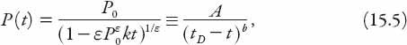
with the restriction on
t
being

Equation (15.5) is in precisely the form stated at the beginning of this subsection.

Exercise:
Derive the solution (15.5).

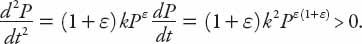
Before we examine some of the implications of this solution, and restrictions on it (remember: every equation tells a story), let’s reexamine equation (15.3) and plot the quantity
k
⁻¹
dP/dt
=
P
^1+
ε
≡
r
_i
,
i
= 0, 1, 2, as a function of
P
for the three cases
ε
> 0,
ε
= 0, and −1 <
ε
< 0, respectively. This last inequality ensures that the population growth rate for this case is not declining, since

In
Figure 15.1
these values correspond to the top, middle, and bottom curves. The case
ε
= 0 (dashed line) clearly corresponds to the equation for exponential growth we have already seen (equation (15.2)). The upper curve corresponds to the arbitrary (and for illustrative purposes, rather large) value for
ε
of 0.5.

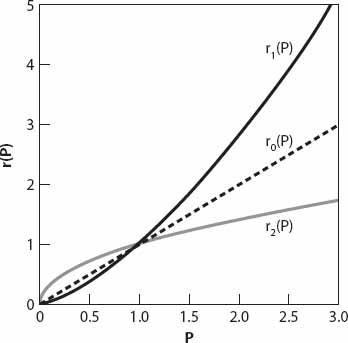
Figure 15.1. Curves proportional to the growth rates for super-exponential, exponential, and sub-exponential growth (from equation (15.3)).

The lower curve has
ε
= −0.5. Now let’s consider a much smaller but positive value of
ε
, 0.05 say. Then the growth is just slightly “super-exponential” with the right-hand side of equation (15.3) increasing in proportion to
P
^1.05
. From equation (15.5) the solution is

This solution is undefined (“blows up”!) at time

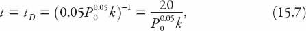
in whatever units of time are being used (usually years, of course). This doomsday time is the
finite
time for the population to become unbounded. Thus if we take the current “global village” world population of 7 billion (as declared on October 31, 2011) to be
P
₀
, and, for simplicity, an annual growth rate
k
= 0.01 yr
⁻¹
(just 1% per year) then for the (admittedly arbitrary) value
ε
= 0.15, equation (15.7) gives

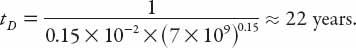
This is the doomsday time for our chosen value of
ε
! Note that if
ε
≤ 0 the problem does not arise because there is no singularity in the solution. The population will still tend to infinity, but will not become infinite in a finite time, as is predicted for
any ε
> 0,
no matter how small
. The original “doomsday” paper [
28
] (and others listed in the references) should be consulted for the specific demographic data used.

Despite such a projection, I thought there was no suggestion that the world population is actually growing according to equation (15.3) until I read a paper [
29
] published in 2001. The first two sentences from the abstract of that paper may serve to whet the reader’s appetite for further discussion later in this book (
Chapter 18
): “Contrary to common belief, both the Earth’s human population and its economic output have grown faster than exponential, that is, in a super-Malthusian mode, for most of known history. These growth rates are compatible with a spontaneous singularity occurring at the same critical time 2052±10 signaling an abrupt transition to a new regime.” Doomsday again?

Exercise:
Obviously the choice
ε
= 0 in equation (15.3) results in the standard exponential growth of
P
as noted above. Using a limiting procedure in equation (15.5), show that

Exercise:
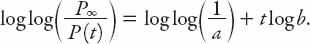
Another model, the “double exponential” model of bounded population growth, is defined by

where
P
_∞
is the asymptotic population (approached as
t
→ ∞), 0 <
b
< 1, and 0 <
a
< 1.

(i) Show that