X and the City: Modeling Aspects of Urban Life (43 page)

  (ii) A town population starts at
P
(0) = 80,000 and has an upper bound
P
_∞
= 200,000. It is known that after 10 years the population has risen to 150,000. Determine the constants
a
and
b
.

 (iii) Find the population after 15 years.

Now we shall discuss a population model that predicts a definite limit on growth. Let’s examine the logistic differential equation

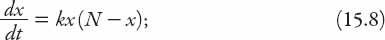
both
k
and
N
are positive constants. We have changed the dependent variable from
P
to
x
to reflect the fact that these models can apply to many different things.
N
is often called the carrying capacity in ecological contexts and the saturation level in chemistry. It can be used to describe, in a very simple
manner, the spread of diseases or rumors in a closed community of population
N
, or a cultural fad, or indeed the spread of anything that can be spread by casual person-to-person contact, from the common cold to word-of mouth advertising about a new brand of coffee! (See
Appendix 8
.) The variable
x
(
t
) describes the number of individuals with the disease, or who have heard the rumor, read the ad, and so on, and for our purposes the most relevant range of values for
x
is 0 <
x
<
N
. The case
x
>
N
is also easily accommodated and will be discussed below. Equation (15.8) is separable, and using partial fractions we can integrate it to obtain

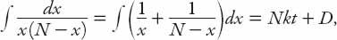
D
being a constant of integration to be determined. Hence

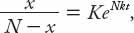
where we have defined
K
=
e
^D
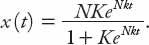
. The general solution
x
(
t
) is therefore

Now rumors don’t start and diseases don’t spread without someone to initiate them, so we define the initial value of
x
to be
x
(0) =
x
₀
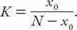
> 0. This enables us to find
K
in terms of the (in principle known) quantities
x
₀
and
N
. Thus

On rearranging the final result, the solution becomes

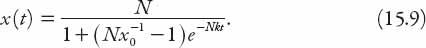
Check that the initial condition is satisfied, and note also that lim
_t
→
∞
x
(
t
) =
N
. This means that
x
=
N
is a horizontal asymptote; if nothing else changes, then the population
x
approaches the limiting value
N
from below (in this case) as time increases. Note that the solution (15.9) is still valid if
x
₀
>
N
; now the solution decreases monotonically from its initial value toward the asymptote from above. This case is meaningless in the present context, though it can apply
to a simple model of overpopulation when the natural resources in a nature reserve, say, become compromised, perhaps by pollution or an environmental disaster. Then the normally sustainable population can no longer be supported, and the numbers decrease toward the
new
carrying capacity.

Further information about the evolution of
x
(
t
) may readily be found from examining both its population growth rate and its
per capita
growth rate using equation (15.8). The latter rate is just

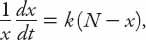
and clearly in the interval 0 <
x
<
N
this is a linearly decreasing function. This means that the per capita growth rate slows uniformly from a maximum near
kN
(when
x
is small) toward zero as the carrying capacity (or saturation level) is approached. On the other hand, it can be seen from equation (15.8) that the population growth rate
dx
/
dt
as a function of
x
is a downward facing parabola with intercepts at
x
= 0,
N
and a maximum of
kN
²
/4 at
x
=
N
/2.

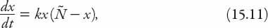
We can now change the context somewhat from the spread of rumors and diseases to a city-related version of harvesting or fishing. Suppose that a city has a problem with vermin—whether of the four-legged, six-legged (bed bugs!), or winged variety (e.g., pigeons), and a program is introduced to reduce the population of these unwanted “critters.” How might we incorporate this “vermin reduction program” into the equations we have been discussing above? We can do this mathematically in two straightforward ways, depending on how the program is administered: by including a constant reduction rate or including a term proportional to the
existing
vermin population. Were we to replace “vermin” by “fish” then we would note that the former more appropriately describes a fishing effort in which the rate at which fish are caught on each fishing foray is the same. In the latter case the catch rate is proportional to the population, and the number of fish caught will thus diminish or increase as the population does. Taking the latter case first because it is mathematically simpler, and possibly more relevant to a town or city with a vermin problem, we can modify equation (15.8) as

Here the term
cx
represents the vermin reduction rate (in units of e.g. rats/week). The constant
c
can be thought of as the per capita reduction rate (rat?) resulting from the program. Noting that equation (15.10) may be rewritten as