X and the City: Modeling Aspects of Urban Life (21 page)

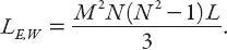
Assuming a uniform demand at the
MN
starting points, each of which serves the
MN
− 1 others, there are
MN
(
MN
− 1) trips, so the average length of all eastbound and westbound trips is

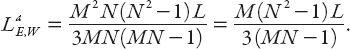
By interchanging
M
and
N
we obtain the corresponding result for N-S trips, that is,

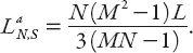
Any single trip will generally involve a combination of both types of trip, so the average length over all trips is

This gratifying result shows that the average trip length is one sixth of the perimeter of the area served, and if the area is square, this is two thirds of the length of a side.

With this general result established (though only for the in-vehicle part of the trip), we proceed with the “walk, wait, ride, and walk” overall trip time calculations for a square city of side
c
. With a grid containing
n
²
equally spaced stations, the distance between adjacent stops is
c
/
n
, and with each station centrally located in its “sub-square,” the average walk distance is, from our earlier discussion,
c
/2
n
, which of course must be doubled for the assumed symmetry of the trip. The time to walk both such trips is
c
/
nW
.

The “wait time” depends on the spacing of the vehicles on a line. For example, if they are two stations apart the wait time is 2
c
/
nV
_a
, and in general,
sc
/
nV
_a
for a vehicle spacing of
s
stations. The trip time is merely the average distance divided by
V
_a
, and from the previous discussion, this will be 2
c
/3
V
_a
. There is also a transfer time for travel involving different vehicles, which for our purposes is just the waiting time multiplied by a factor
F
of order one. (There are data [
14
] indicating that for networks sizes up to 10 × 10, 0.5 ≤
F
≤ 2. This will be generically incorporated in the term
sc
/
nV
_a
for the calculations below.)

Combining all three “times,” that is, walk + wait + in-vehicle, we express the overall trip time as

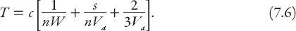
In keeping with the literature [
14
], we choose a city size of
c
= 10 km. In Europe, typical population densities are around [
14
] 4000/km
²
(the average figure for U.S. cities is about half this). Thus “our” city has a population of about 400,000. The average length of all trips is, as noted above, 2/3 of the side length, approximately 6.7 km. Again, fictionally treating the station spacing as a continuous variable, we can the network travel time as a function of station spacing from the above formula.

The total travel time in minutes is shown in
Figure 7.4
for
V
_m
= 30 km/hr (upper curve) and 80 km/hr (middle curve). The lower (dotted) line is the
walk time, and it can be seen that the walk time is the dominant contribution for large station spacing (corresponding to fewer tracks). Notice that the minimum travel time for the slower speed of 30 km/hr occurs at a stop spacing of about 0.25 km (appropriate for a city bus route) and at about 0.5 km for the 80 km/hr monorail route.

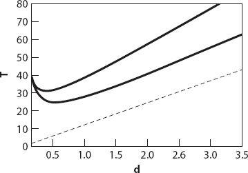
Figure 7.4. Total travel time (minutes) vs. stop spacing for a maximum speed of 30 km/hr (upper curve) and 80 km/hr (middle curve). The dotted line represents the walk time component for one end of the trip.

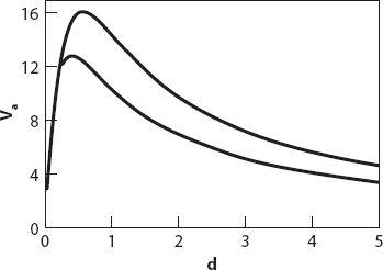
Figure 7.5. Average speeds in km/hr vs. stop spacing, based on
Figure 7.4
. The upper curve is for a maximum speed of 80 km/hr, the lower for a maximum speed of 30 km/hr.

Figure 7.5
shows the average speed for these curves (starting for
d
=
L
= 0.1 km). Note that the maximum average speed is only between about 13 and 16 km/hr for the range of maximum speeds considered here.

The much higher value for
V
_m
of 80 km/hr adds relatively little to the average speed.

A final word:
pedestrians
. The most complete forms of the above models make allowances for the average time to walk to and from the station. As someone who has walked to work almost every weekday for twenty-eight years, I have learned to be very careful about crossing roads. I have to judge whether there is sufficient time to do so before the nearest vehicle reaches me. (One certainly hopes there is.) In fact, every individual has (in principle) a
critical time gap
,
T
say, above which crossing is acceptable and below which it is not. Mathematically, this can be represented by a step function

G
(
t
) = 0,
t
≤
T
,
G
(
t
) = 1,
t
>
T
.

I think a step function is an entirely appropriate thing for pedestrians to have.

As noted in the previous chapter, in many very large cities a car is not needed at all. But there also are many cities and towns where it is essential to have a vehicle. One advantage of driving over public transportation can be that one does not have to keep stopping at intermediate locations on the way to one’s destination (traffic permitting). Of course, the daily commute can be extremely frustrating when it is of the stop-and-start variety, and the gas consumption becomes prohibitive. At the time of writing the price of petrol in the UK is far higher (by a factor of two) than the equivalent cost of gas in the U.S. It must be the different spelling that causes this. But before discussing that and other driving-related topics, let’s start with an unrealistic but amusing and informative question.