X and the City: Modeling Aspects of Urban Life (19 page)

but for physical reasons we require only those solutions that tend to zero as
z
→ ∞. The two satisfying this condition are those for which Re
σ
< 0,

Using these roots, the temperature solution (6.9) can be expressed in terms of (complex) constants
c
₁
and
c
₂
as

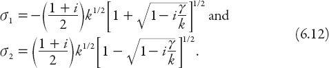
Note from equation (6.12) that
Using specified boundary conditions, both
c
₁
and
c
₂
can be expressed entirely in terms of
σ
₁
and
σ
₂
, though we shall do not do so here. The authors note typical magnitudes for the parameters describing the heat island of a large city (based on data for New York City). The diameter of the heat island is about 20 km, with a surface value for Δ
T
≈ 2
C
, and a mean wind speed of 3 m/s.

Exercise:
Verify the results (6.10)–(6.12).

As we have remarked already, cities come in many shapes and sizes. In many large cities such as London and New York, the public transportation system is so good that one can get easily from almost anywhere to anywhere else in the city without using a car. Indeed, under these circumstances a car can be something of an encumbrance, especially if one lives in a restricted parking zone. So for this chapter we’ll travel by bus, subway, train, or quite possibly,
rickshaw. Whichever we use, the discussion will be kept quite general. But first we examine a situation that can be more frustrating than amusing if you are the one waiting for the bus.

In a delightful book entitled
Why Do Buses Come in Threes?
[
8
] the authors suggest that in fact, despite the popular saying, buses are more likely to come in twos. Here’s why: even if buses leave the terminal at regular intervals, passengers waiting at the bus stops tend to have arrived randomly in time. Therefore an arriving bus may have (i) very few passengers to pick up, and little time is lost, and it’s on its way to the next stop, or (ii) quite a lot of passengers to board. In the latter case, time may be lost, and the next bus to leave the terminal may have caught up somewhat on this one. Furthermore, by the time it reaches the next stop there may be fewer passengers in view of the group that boarded the previous bus, so it loses little time and moves on. For the next two buses, the cycle may well repeat; this increases the likelihood that buses will tend to bunch in twos, not threes.

The authors note further that
if
a group of three buses occurs at all (and surely it sometimes must), it is most likely to do so near the end of a long bus route, or if the buses start their journeys close together. So let’s suppose that they do . . . that they leave the terminal every
T
minutes, and that once they “get their buses in a bunch” buses
A
and
B
and
B
and
C
are separated by
t
minutes (where
t
<
T
of course). A fourth bus leaves
T
minutes after
C
, and so on. The four buses have a total of 3
T
minutes between them, initially at least. When the first three are bunched up, the fourth bus is 3
T
− 2
t
minutes behind
C
(other things such as speed and traffic conditions being equal). If you just missed the first or the second bus, you have a wait of
t
minutes for the third one; if you just missed that then you have a wait of 3
T
− 2
t
minutes. Thus your average wait time under these circumstances is just
T
, the original gap between successive buses!

How does this compare with
not
missing the bus? The probability that you have arrived in the long gap as opposed to one of the two short ones is (3
T
− 2
t
)/3
T
, your time of arrival could be just after the third bus left, just before the fourth one arrives, or any time in between, and the mean of those two extremes is (0 + 3
T
− 2
t
)/2. This will actually be longer than the previous
average wait time if
T
> 2
t
, which of course is quite likely, even allowing for the small possibility that you arrived in a
t
-minute gap.

We shall examine and “unpack” an idealized analysis of public transport systems (based on an article [
14
] published in the transportation literature). The article contained a comprehensive account of two models: a corridor system and a network system. In so doing, it is possible to derive some general results for transport systems. Although some of these conclusions were represented in graphical form only, the mathematics behind those graphs is well worth unfolding here. In both models there are three components to the travel time from origin
A
to destination
B
: (i) the walk times to and from the station at either end; (ii) the time waiting for the transportation to arrive; and (iii) the total time taken by the subway train, bus, or train to go from the station nearest
A
(
S
_A
) to that nearest
B
(
S
_B
). (This includes waiting time at intermediate stops along the way.)

In what follows, the city is assumed to have a “grid” system with roads running N-S and E-W (see
Appendix 3
on “Taxicab geometry”). While this may be more appropriate to cities in the United States, it is also an acceptable approximation for many European cities [
14
], [
15
]. From
Figure 7.1
we see that a walk from any location to any station will involve an N-S piece and an E-W piece. If each station is considered to be at the center of a square of side
L
,
the average walk length is
L
/2. To see this, note that for any trip starting at the point (
x
,
y
) on the diagonal line (for which
x
+
y
=
L
/2) to the center is just
L
/2. By symmetry, there is the same area on each side of the line. If the population demand is uniformly distributed,
L
/2 is the average trip to or from the central station, and hence
L
is the average total distance walked—just the average stop separation.

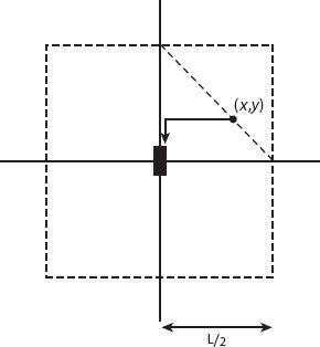
Figure 7.1. One segment of a transportation corridor with a central station serving a square area of side
L
. The diagonal shown has equation
x
+
y
=
L
/2.

First we consider the average speed
V
_a
for the vehicular part of the trip. We suppose that this part consists of a uniform acceleration
a
from rest to a (specified) maximum speed
V
_m
(
A
–
B
), and a period of travel at this speed (
B
–
C
–
D
) followed by a uniform deceleration −
a
to rest at the next station (
D
–
E
). The acceleration and deceleration take place over a distance
x
km, say, and the speed is constant for a distance
L
− 2
x
≥ 0. Using the equations of motion for uniform acceleration it is found that
V
_m
= (2
ax
)
^1/2
and the time
T
_x
to travel the distance
x
(= distance
AB
) and reach this maximum speed is
T
_x
= (2
x
/
a
)
^1/2
. The time to travel the distance
BC
is therefore
T
_BC
= ([
L
/2] −
x
)/
V
_m
. If we include a waiting time
T
_W
at the station
A
before leaving for the next one at
E
, the total time for the journey
AE
is 2 (
T
_x
+
T
_BC
) +
T
_W
; typically,
T
_W
≈ 20s and
a
= 0.1
g
according to published data [
15
]. Hence the average speed in terms of the maximum speed is