X and the City: Modeling Aspects of Urban Life (22 page)

X
=
: GASOLINE CONSUMPTION IN THE CITY

Question:
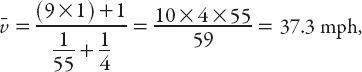
A car travels from a home in the suburbs to a downtown office building, somehow maintaining a constant speed of 30 mph. On the return journey it maintains a constant speed of 60 mph. What is its average speed?

No, it’s not 45 mph, sorry. The car spends twice as long traveling at 30 mph as it does returning at 60 mph, so the average speed will be “weighted” toward the lower speed. The correct answer is 40 mph. To see why, the average speed is defined as the total distance traveled divided by the total time (
T
) for the round trip. For those who are concerned that we have not specified the distance from the proverbial “
A
to
B
”—not to worry, let’s just call it
d
. Then the average speed is

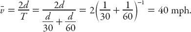
In fact, the above result is the
harmonic mean
of the two speeds. The harmonic mean of a set of numbers is the reciprocal of the arithmetic mean of the reciprocals! Put more obviously in mathematical terms, for a set of
n
numbers
x
_i
,
i
= 1, 2, 3, . . . 
n
, the harmonic mean
H
is

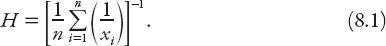
That’s the power of algebra for you! The incorrect answer of 45 mph is based on the arithmetic mean, which as we see, is not the appropriate measure of “average” for this problem. This difference is exacerbated by considering more than one “vehicle”; suppose that nine vehicles traverse a route one mile in length, and that all travel at the posted speed limit of 55 mph. I decide to walk the route at a reasonable pace, say 4 mph. The average speed for all ten trips, as computed by using the arithmetic mean is

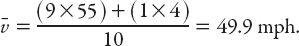
On the other hand, if we calculate the total distance traveled and divide it by the total time taken, the result is

a considerable difference.

Question:
If we replace “speed” by “average speed” in the above question, does it change the result?

Exercise:
Generalize the first result for speeds
v
₁
and
v
₂
.

X
= Δ
E
: Question:
How does gasoline consumption vary with speed?

In recent years, as well as several decades ago, the increasing costs of oil and gasoline have threatened to change the habits of American motorists, and in some cases has done so (albeit for a limited period of time, after which gas prices have declined, and everything reverts to the
status quo
). We know that at low speeds in low gears fuel consumption rate is relatively high because of lower efficiency in converting chemical energy to kinetic energy at these speeds. At high speeds the effects of air resistance (or drag) also increases the rate of fuel consumption. So it’s certainly reasonable to conclude that there is an optimal speed (or range of speeds) for which the rate of fuel consumption is minimized.

The national 55-mph speed limit in the U.S. is no longer in existence, but in 1982 a newspaper article stated that one should “Observe the 55-mile-an-hour national highway speed limit.” Furthermore, it stated that “For every five miles an hour over 50, there is a loss of one mile to the gallon. Insisting that drivers stay at the 55-mile-an-hour mark has cut fuel consumption 12 percent for [Company name] of Jacksonville, Florida—a savings of 631,000 gallons of fuel a year. The most fuel-efficient range for driving generally is considered to be between 35 and 45 miles an hour” (“Boost Fuel Economy,”
Monterey Peninsula Herald
, May 16, 1982, as quoted in Giordano et al. 2003).

My first reaction on reading this was to wonder if the article is referring to fuel consumption for domestic as opposed to commercial vehicles, or both (which seems unlikely). And I very much doubt that the mpg losses are a linear function of speed above 55 mph as suggested. Surely there are more factors that affect how many miles per gallon we get from our vehicles, such as the age
of the engine (and maybe the driver!), the type of fuel used, the air temperature, the speed of travel, and the resistive forces of drag and road friction. Drag will depend on the speed and shape of the vehicle and the prevailing atmospheric conditions at the ground (wind in particular). Friction will depend on the condition of the tires, and the type and weight of the car. The nature of the terrain is very important also: is it a flat, smooth road or an unpaved track in a hilly or mountainous region? How good is the driver? Does he drive smoothly where possible, or speed up/slow down in an irregular pattern, even if the road conditions do not warrant it? Is she an experienced driver or a novice? These and probably several other considerations all have bearing on the problem of interest here.

The drag force on most everyday objects is proportional to their cross-sectional area
A
and the square of their speed
v
. Therefore driving at highway speeds for a distance
d
will consume energy
E
∝
Av
²
d
. For a given value of
d
and a small change in
v
(Δ
v
), the corresponding percentage change in energy expended is [
16
]

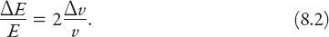
While the change from driving at 70 mph (as many do) to 60 mph (about 14%) may not be considered “small,” we’ll use it anyway, and conclude that there is a nearly 30% drop in fuel consumption. This makes a lot of sense!

What thoughts typically run through your mind as you approach a traffic signal? Here are some likely ones: will it stay green long enough for me to continue through? Will it turn red in enough time for me to stop? What if it turns yellow and someone is close behind me—should I try to stop or go through? And perhaps related to the latter thought, “Is there a police car in the vicinity?”

Obviously we assume that the car is being driven at or below the legal speed. If the light turns yellow as you approach the signal you have a choice to make: to brake hard enough to stop before the intersection, or to accelerate (or coast)
and continue through the intersection legally before the light turns red. Unfortunately, many accidents are caused by drivers misjudging the latter (or going too fast) and running a red light.

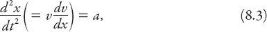
The mathematics involved in describing the limits of legal maneuvers is straightforward: integration of Newton’s second law of motion. Suppose that the width of the intersection is
s
ft and that at the start of the deceleration (or acceleration), time
t
= 0, and the vehicle is a distance
d
₀
from the intersection and traveling at speed
v
₀
. If the duration of the yellow light is
T
seconds, and the
maximum
acceleration and deceleration are denoted by
a
₊
and −
a
₋
respectively, then we have all the initial information we need to find expressions for the two situations above: to stop or continue through. A suitable form of Newton’s second law relates displacement
x
and acceleration
a
as