X and the City: Modeling Aspects of Urban Life (57 page)

For any given
x
> 0 this will have its maximum value when
y
= 0, so it will be of interest to determine the location of the maximum of the function

Using the first derivative test it is straightforward to show that the maximum ground-level concentration of

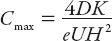
at
x
=
x
_m
=
UH
²
/4
D
. Using this very simple model we have been able to reproduce a result first derived in 1936 [
34
], namely that the maximum ground-level concentration from a plume released from a height
H
is inversely proportional to
H
²
.

Exercise:
Verify this result.

Summarizing, therefore, the model predicts that

  I.
C
_max
is inversely proportional to the square of the plume-release height
H
.

  II.
C
_max
is inversely proportional to the wind speed
U
.

 III.
x
_m
is directly proportional to the square of the plume-release height
H
.

 IV.
x
_m
is directly proportional to the wind speed
U
.

  V.
C
_max
and
x
_m
are both independent of the ground “reflection coefficient”
α
.

The model developed here is very simplistic, so it is encouraging to note that the first two predictions are the same as those from more sophisticated models. Physically, they make sense, since the plume is diffusing in both the
y
- and
z
-directions as the wind carries it downstream, and the pollutants are spread over a wider area (which has dimensions of (length)
²
). Furthermore, a stronger wind will stretch out the plume more per unit time, diluting it all the more as it does so.

As for the remaining predictions, III and IV follow naturally for the same reasons as I and II. In reality, the effect of ground reflection must play a role, though perhaps only a minor one compared to that of
H
and
U
. One mechanism neglected here is that of
buoyancy
; very often the effluents released (or, indeed, smoke from forest fires) is warmer than the surrounding air, and it continues to rise for a time after it is released. But to keep things relatively simple, that effect has not been included here.

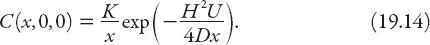
We have regarded the source of effluent to be on the ground or at the top of a smokestack. In each case the source is in effect a
point source
. This is because of
the nature of the solution at
x
= 0, referred to above. But consider a long line of slowly moving bumper-to-bumper traffic along a straight stretch of road. This can be considered a distributed source of particulates (current emission regulations notwithstanding)—a
line source
. Of course, the average speed of the traffic, the length of the road, and the wind strength and direction will affect the concentration of particles (such as hydrocarbons from the tailpipes) at any point on or off the road. To build a simple model of pollutant dispersal for a line of traffic of length
L
, we now use the emission rate per unit length, namely
K
/
L
. We will again neglect buoyancy and regard the line source as being placed at ground level along the
y
-axis from −
L
/2 to
L
/2 (though it is not necessary to specify this in what follows). We shall utilize the earlier models by considering only a cross-wind
U
in the
x
-direction as before; thus the pollutant is blown directly from the road into the neighboring land or cityscape. For a long traffic line
L
(strictly, an infinitely long line) there can be no variation of
C
in the
y
-direction because the source is uniform along that line. Therefore we approximate the finite-
L
case by requiring that the particles diffuse only in the vertical direction (again, the effect of wind dominates any diffusion in the
x-
direction). The governing equation now simplifies to

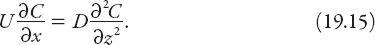
Again, dropping the subscript, this time on
K
₁
, the solution, based on equation (19.9), is now

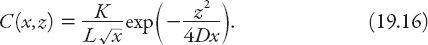
Note that at ground level (
z
= 0) the concentration varies more slowly downwind, as
x
^−1/2
, compared with
x
⁻¹
for a point source. Clearly the concentration for any
x
> 0 is maximized at ground level, but this result is a means to an end. In many situations, the source will be better approximated, not by a point or a line, but by an
area
composed of multiple sources in an urban region. These can effectively combine because of wind and diffusion in such a way as to render the individual sources unidentifiable. Since we are interested in the ground-level concentration, we set
z
= 0 in the above equation and imagine for simplicity a
rectangular
source by integrating the result with respect to
x
. Therefore the accumulated concentration
C
_A
(
x
) has the following dependence on
x
:

More realistic models indicate a greater dependence on
x
than this, especially if the atmospheric conditions preclude the particles from unlimited diffusion vertically. There is evidence to suggest that the rate at which pollutants are emitted and the region affected by pollution both increase faster than the population does. Modeling this would be a very substantial exercise for the reader!

With such particles suspended in the atmosphere for sometimes days or weeks at a time, smog presents a danger to health, but in London it was also known as a “pea souper” because one could not see one’s hand in front of one’s face! In fact, as a result of the Great London Smog of 1952 (caused by the smoke from millions of chimneys combined with the mists and fogs of the Thames valley), the Clean Air Act of 1956 was enacted. With this in mind we now turn to the topic of how air pollution may affect
visibility
.

We start with an apparent
non sequitur
by asking the following question. Have you ever been in an auditorium of some kind, or a church, in which your view of
a speaker is blocked by a pillar, but you can still hear what is being said? I’m pretty sure you must have experienced this. Why can your ears receive auditory signals, but your eyes cannot receive direct visual ones (excluding Superman of course)? The reason for this is related to the wavelengths of the sound and light waves, being ≈1m and ≈5 × 10
⁻⁷
m, respectively. The latter, in effect, “scatter” more like particles while the former are able to diffract (“bend”) around an obstacle comparable in size to their wavelength. By the same token, therefore, we would expect that light waves can diffract around appropriately smaller obstacles, and indeed this is the case, as evidenced by softly colored rings of light around the moon (coronae) as thin cloud scuds past its face. Another diffraction-induced meteorological phenomenon is the green, purple-red, or blue iridescence occasionally visible in clouds. But it is the collective phenomenon known as
scattering
that we wish to discuss in some detail, in order to better appreciate the character of air pollution and its effect on the light that reaches our eyes.