Statistics Essentials For Dummies (40 page)

Finding critical values

If you don't know the population standard deviation and are using the sample standard deviation instead, you pay a penalty: a t-distribution with more variability and fatter tails. When you do a hypothesis test, your "cutoff point" for rejecting the null hypothesis H
_o
is further out than it would have been if you had more data and could use the Z-distribution. (For more information on hypothesis tests and how they are set up, see Chapter 8.)

For example, suppose you have a two-tailed hypothesis test for one population mean where
= 0.05 and you have a sample size of 100. If you are doing a two-sided hypothesis test for one population mean, you can use Z = plus or minus 1.96 as your critical value to determine whether to reject H
_o
. But if
n
is, say, 8, the critical value for this same test would be t
₇
= plus or minus 2.365 ; see Table A-2, row 7, column "0.025" to obtain this number. (Remember a two-tailed hypothesis test with significance level 5% has 2.5% = 0.025 in each tail area.) This means you have to submit more evidence to reject Ho if you only have 8 pieces of data than if you have 100 pieces of data. In other words, your goal line to make a touchdown and find a "statistically significant result" is set at 2.365 for the
t-
distribution versus 1.96 for the
Z-
distribution.

Finding p-values

Recall from hypothesis testing (Chapter 8) that a
p
-value is the probability of obtaining a result beyond your test statistic on the appropriate distribution. In terms of
p
-values, the same test statistic has a larger
p
-value on a
t-
distribution than on the
Z-
distribution. A test statistic far out on the leaner
Z-
distribution has little area beyond it. But that same test statistic out on the fatter
t-
distribution has more fat (or area) beyond it, and that's exactly what the
p
-value represents.

Suppose your sample size is 10, your test statistic (referred to as the
t-value
) is 2.5, and your alternative hypothesis, H
_a
, is the greater-than alternative. Because the sample size is 10, you use the
t-
distribution with 10 - 1 = 9 degrees of freedom to calculate your
p
-value. This means you'll be looking at the row in the
t-
table (Table A-2 in the Appendix) that has a 9 in the Degrees of Freedom column. Your test statistic (2.5) falls between two values: 2.262 (the "0.025" column) and 2.821 (the "0.01" column). The
p
-value is between 0.025 = 2.5% and 0.01 = 1%. You don't know exactly what the
p
-value is, but because 1% and 2.5 % are both less than the typical cutoff of 5%, you reject H
_o
.

The
t-
table (Table A-2 in the Appendix) doesn't include all possible test statistics on it, so simply choose the one test statistic that's closest to yours, look at the column it's in, and find the corresponding percentile. Then figure your
p
-value.

Note that for a less-than alternative hypothesis, your test statistic would be a negative number (to the left of 0 on the
t-
distribution). In this case, you want to find the percentage below, or to the left of, your test statistic to get your
p
-value. Yet negative test statistics don't appear on Table A-2. Not to worry! The percentage to the left (below) a negative
t-
value is the same as the percentage to the right (above) the positive
t-
value, due to symmetry. So, to find the
p
-value for your negative test statistic, look up the positive version of your test statistic in Table A-2, and find the corresponding right tail probability. For example, if your test statistic is -2.5 with 9 degrees of freedom, look up +2.5 on Table A-2, and you find that it falls between the 0.025 and 0.01 columns, so your
p
-value is somewhere between 1% and 2.5%.

If your alternative hypothesis (H
_a
) has the no
t-
equal-to alternative, double the percentage that you get to obtain your
p
-value. That's because the
p
-value is this case represents the chance of being beyond your test statistic in either the positive or negative direction (see Chapter 8 for details on hypothesis testing).

t-distributions and Confidence Intervals

The
t-
distribution is used in a similar way with confidence intervals (see Chapter 7 for more on confidence intervals.) If your data have a normal distribution and either 1) the sample size is small; or 2) you don't know the population standard deviation,
, and you must use the sample standard deviation,
s
, to substitute for it, you use a value from a
t-
distribution with
n
- 1 degrees of freedom instead of a
z-
value in your formulas for the confidence intervals for the population mean.

For example, to make a 95% confidence interval for
where
n
= 9 you add and subtract 2.306 times the standard error of
when you use the
t-
distribution versus adding and subtracting 1.96 times the standard error when you use a
z-
value.

Chapter 10
:
Correlation and Regression

In This Chapter

Exploring statistical relationships between numerical variables

Distinguishing between association, correlation, and causation

Making predictions based on known relationships

In this chapter you analyze two numerical variables,
X
and
Y
, to look for patterns, find the correlation, and make predictions about
Y
from
X
, if appropriate, using simple linear regression.

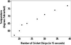
Picturing the Relationship with a Scatterplot

A fair amount of research supports the claim that the frequency of cricket chirps is related to temperature. And this relationship is actually used at times to predict the temperature using the number of times the crickets chirp per 15 seconds. To illustrate, I've taken a subset of some of the data that's been collected on this; you can see it in Table 10-1.

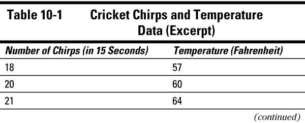
Notice that each observation is composed of two variables that are tied together, in this case the number of times the cricket chirped in 15 seconds (the
X
-variable), and the temperature at the time the data was collected (the
Y
-variable). Statisticians call this type of two-dimensional data
bivariate
data. Each observation contains one pair of data collected simultaneously.

Making a scatterplot

Bivariate data are typically organized in a graph that statisticians call a
scatterplot.
A scatterplot has two dimensions, a horizontal dimension (called the
x
-axis) and a vertical dimension (called the
y
-axis). Both axes are numerical — each contains a number line.

The
x
-coordinate of bivariate data corresponds to the first piece of data in the pair; the
y
-coordinate corresponds to the second piece of data in the pair. If you intersect the two coordinates, you can graph the pair of data on a scatterplot. Figure 10-1 shows a scatterplot of the data from Table 10-1.

Interpreting a scatterplot

You interpret a scatterplot by looking for trends in the data as you go from left to right:

If the data show an uphill pattern as you move from left to right, this indicates a
positive relationship between X and Y.
As the
x-
values increase (move right), the
y
-values increase (move up) a certain amount.

If the data show a downhill pattern as you move from left to right, this indicates a
negative relationship between X and Y.
That means as the
x
-values
increase (move right) the
y
-values decrease (move down) by a certain amount.

If the data don't resemble any kind of pattern (even a vague one), then no relationship exists between
X
and
Y
.

This chapter focuses on linear relationships. A
linear relationship between X and Y
exists when the pattern of
x
- and
y
-values resembles a line, either uphill (with positive slope) or downhill (with negative slope).

Looking at Figure 10-1, there does appear to be a positive linear relationship between number of cricket chirps and the temperature. That is, as the cricket chirps increase, you can predict that the temperature is higher as well.