Statistics Essentials For Dummies (39 page)

Perhaps your sample, while collected randomly, just happens to be one of those atypical samples whose result ended up far out on the distribution. So H
_o
could be true, but your results lead you to a different conclusion. How often does that happen? Five percent of the time (or whatever your given alpha level is for rejecting H
_o
).

A missed detection: Type-2 error

Now suppose the company really wasn't delivering on its claim. Who's to say that the consumer group's sample will detect it? If the actual delivery time is 2.1 days instead of 2 days, the difference would be pretty hard to detect. If the actual delivery time is 3 days, a fairly small sample would show that something's up. The issue lies with those in-between values, like 2.5 days. If H
_o
is indeed false, you want to detect that and reject H
_o
. Not rejecting H
_o
when you should have is called a
Type-2 error.
I call it a
missed detection.

Sample size is the key to being able to detect situations where H
_o
is false and to avoiding Type-2 errors. The more information you have, the less variable your results will be, and easier it will be to detect problems that exist with a claim.

This ability to detect when H
_o
is truly false is called the
power
of a test. Power is a pretty complicated issue, but what's important for you to know is that the higher the sample size, the more powerful a test is. A powerful test has a small chance for a Type-2 error.

Statisticians recommend two preventative measures to minimize the chances of a Type-1 or Type-2 error:

Set a low cutoff probability for rejecting H
_o
(like 5 percent or 1 percent) to reduce the chance of false alarms (minimizing Type-1 errors).

Select a large sample size to ensure that any differences or departures that really exist won't be missed (minimizing Type-2 errors).

Chapter 9
:
The t-distribution

In This Chapter

Characteristics of the
t-
distribution

Relationship between
Z-
and
t-
distributions

Understanding the
t-
table

Many different distributions exist in statistics, and one of the most commonly used distributions is the
t-
distribution. In this chapter I go over the basic characteristics of the
t-
distribution, how to use the
t-
table to find probabilities, and how it's used to solve problems in its most well-known settings — confidence intervals and hypothesis tests.

Basics of the t-Distribution

The normal distribution is the well-known bell-shaped distribution whose mean is
and whose standard deviation is
. (See Chapter 5 for more on normal distributions.) The
t-
distribution can be thought of as a cousin of the normal distribution — it looks similar to a normal distribution in that it has a basic bell shape with an area of 1 under it, but is shorter and flatter than a normal distribution. Like the standard normal (Z) distribution, it is centered at zero, but its standard deviation is proportionally larger compared to the
Z-
distribution.

As with normal distributions, there is an entire family of different
t-
distributions. Each
t-
distribution is distinguished by what statisticians call
degrees of freedom
, which are related to the sample size of the data set. If your sample size is
n
, the degrees of freedom for the corresponding
t-
distribution is
n
- 1. For example, if your sample size is 10, you use a
t-
distribution with 10 - 1 or 9 degrees of freedom, denoted t9.

Smaller sample sizes have flatter
t-
distributions than larger sample sizes. And as you may expect, the larger the sample size is, and the larger the degrees of freedom, the more the
t-
distribution looks like a standard normal distribution (
Z-
distribution); and the point where they become very similar (similar enough for jazz or government work) is about the point where the sample size is 30. (This result is due to the Central Limit Theorem; see Chapter 6.)

Figure 9-1 shows different
t-
distributions for different sample sizes, and how they compare to the Z-distribution.

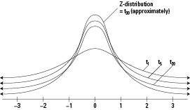
Figure 9-1:
t-
distributions for different sample sizes

Understanding the t-Table

Each
t-
distribution has its own shape and its own set of probabilities, so one size doesn't fit all. To help with this, statisticians have come up with one abbreviated table that you can use to mark off certain points of interest on several different
t-
distributions whose degrees of freedom range from 1 to 30 (see Appendix Table A-2). If you look at the column headings in Table A-2, you see selected values from 0.40 to 0.0005. These numbers represent right tail probabilities (the

probability of being larger than a certain value). The numbers moving down any given column represent the values on each t-distribution having those right tail probabilities. For example, under the "0.05" column, the first number is 6.313752. This represents the number on the
t
1 distribution (one degree of freedom) whose probability to the right equals 0.05. Further down that column in row 15 you see 1.753050. This is the number on the t15 distribution whose probability to the right is 0.05.

You can also use the t-table to find percentiles for the t-distribution (recall that a percentile is a number whose area to the
left
is a given percentage). For example, suppose you have a sample of size 10 and you want to find the 95th percentile. You have n - 1= 9 degrees of freedom, so you look at the row for 9, and the column for 0.05 to get t = 1.833. Since the area to the right of 1.833 is 0.05, that means the area to the left must be 1 - 0.05 = 0.95 or 95%. You have found the 95th percentile of the t9 distribution: 1.833. Now, if we increase the sample size to
n
= 20, the 95th percentile decreases; look at the row for 20 - 1 = 19 degrees of freedom, and in the 0.05 column you find t = 1.729. Remember as
n
gets large, the values on a
t-
distribution are more condensed around the mean, giving it a more curved shape, like the
Z-
distribution.

Notice that as the degrees of freedom of the
t-
distribution increase (as you move down any given column in Table A-2 in the appendix), the
t
-values get smaller and smaller. The last row of the table corresponds to the values on the Z-distribution. That confirms what you already know: As the sample size increases, the
t-
and the
Z-
distributions are more and more alike. The degrees of freedom for the last row of the t-table (Table A-2) are listed as "infinity" to make the point that a t-distribution approaches a Z-distribution as n gets infinitely large.

t-distributions and Hypothesis Tests

The most common use by far of the
t-
distribution is in hypothesis testing — in particular the case where you do a hypothesis test for one population mean. (See Chapter 8 for the whole

scoop on hypothesis testing.) You use a
t-
distribution when you do not know the standard deviation of the population (
) and you have to use the standard deviation of the sample (
s
) to estimate it. Typically in these situations you also have a small sample size (but not always).