101 Excel 2013 Tips, Tricks and Timesavers (30 page)
Read 101 Excel 2013 Tips, Tricks and Timesavers Online
Authors: John Walkenbach

The preceding set of steps uses the column names to create the formula. Alternatively, you can enter the formula by using standard cell references. For example, you can enter the following formula in cell E3:
=D3-C3
If you type the cell references, Excel still automatically copies the formula to other cells in the column.
Referencing data in a table
Formulas that are outside of a table can refer to data within a table by using the table name and column headers. You don’t need to create names for these items. The table itself has a name (for example, Table1), and you can refer to data within the table by using column headers.
You can, of course, use standard cell references to refer to data in a table, but using table references has a distinct advantage: The names adjust automatically if the table size changes by adding or deleting rows.
Refer to the table shown earlier in Figure 75-1. This table was given the name Table1 when it was created. To calculate the sum of all data in the table, use this formula:
=SUM(Table1)
This formula always returns the sum of all the data, even if rows or columns are added or deleted. And, if you change the name of Table1, Excel automatically adjusts formulas that refer to that table. For example, if you rename Table1 as AnnualData (by using the Name Manager), the preceding formula changes to
=SUM(AnnualData)
Most of the time, you want to refer to a specific column in the table. The following formula returns the sum of the data in the Actual column (but ignores the total row):
=SUM(Table1[Actual])
Notice that the column name is enclosed in square brackets. Again, the formula adjusts automatically if you change the text in the column heading.
Even better, Excel provides some helpful assistance when you create a formula that refers to data within a table. Figure 75-4 shows the Formula AutoComplete feature helping to create a formula by showing a list of the elements in the table.
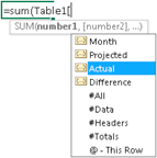
Figure 75-4:
The Formula AutoComplete feature is useful when creating a formula that refers to data in a table.
Tip 76: Numbering Table Rows Automatically
In some situations, you may want a table to include sequential row numbers. This tip describes how to take advantage of the calculated column feature (explained in Tip 75) and create a formula that numbers table rows automatically.
Figure 76-1 shows a table (named
Table1
) with information about job applicants. The first column of the table, labeled
Num
, displays sequential numbers.
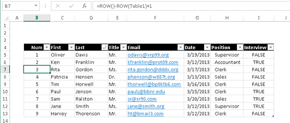
Figure 76-1:
The numbers in column B are generated with a formula.
The calculated column formula, which you can enter into any cell in the
Num
column, is
=ROW()-ROW(Table1)+1
When you enter the formula, it’s automatically propagated to all other cells in the
Num
column.
The ROW function, when used without an argument, returns the row that contains the formula. When the ROW function has an argument that consists of a multirow range, it returns the first row of the range.
 A table’s name does not include the header row of the table. So, in this example, the first row of Table1 is row 5.
The numbers are table row numbers, not numbers that correspond to a particular row of data. For example, if you sort the table, the numbers will remain consecutive — and they will no longer be associated with the same row of data.
If you filter the table, rows that don’t meet the filter criteria will be hidden. In such a case, some table row numbers will not be visible. Figure 76-2 shows the table after filtering to display only the Clerk positions.
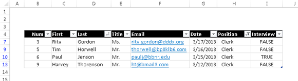
Figure 76-2:
When the table is filtered, the row numbers are no longer consecutive.
If you want the table row numbers to remain consecutive when the table is filtered, a different formula is required. Referring to the example in Figure 76-1, enter this formula in cell B5, and it will be propagated to the other rows:
=SUBTOTAL(3,C$5:C5)
This formula uses the SUBTOTAL function, with a first argument of 3 (which corresponds to COUNTA). The SUBTOTAL function ignores hidden rows, so only visible rows are counted. Notice that the formula refers to a different column — which is necessary to avoid a circular reference error.
Figure 76-3 shows the filtered table using the SUBTOTAL formula in column B.
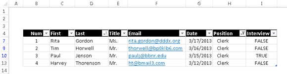
Figure 76-3:
When the table is filtered, the row numbers remain consecutive.
Tip 77: Identifying Data Appropriate for a Pivot Table
A pivot table requires that your data is in the form of a rectangular database table. You can store the database in either a worksheet range (which can be a table or just a normal range) or an external database file. And although Excel can generate a pivot table from any database, not all databases benefit.
Figure 77-1 shows part of a simple database table that has five columns and 3,144 rows (one row for each county). This data is appropriate for a pivot table. For example, a pivot table can instantly calculate the total population by state or by region and display the values in a nicely formatted table.
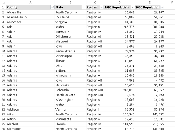
Figure 77-1:
This data is appropriate for a pivot table.
Generally speaking, fields in a database table consist of two types of information:
→
Data:
Contains a value or data to be summarized. For this example, the 1990 Population and the 2000 Population fields are data fields.
→
Category:
Describes the data. For this example, the Country, State, and Region fields are category fields because they describe the two data fields.
The data versus category distinction can be blurry at times. Often a pivot table will display counts of items within a category. In such a case, a category is serving as a data field.
A database table that’s appropriate for a pivot table is said to be normalized. In other words, each row contains information that describes the data in the row.
A single database table can have any number of data fields and category fields. When you create a pivot table, you usually want to summarize one or more of the data fields. Conversely, the values in the category fields appear in the pivot table as rows, columns, or filters.
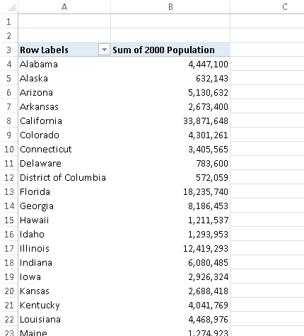
Figure 77-2 shows a pivot table created from the example. This pivot table displays the 2000 Population values, totaled by state.