101 Excel 2013 Tips, Tricks and Timesavers (26 page)

Tip 65: Using Flash Fill to Combine Data

Tip 64 described how to extract data using the Excel 2013 Flash Fill feature. This tip looks at the other side of Flash Fill: combing data.

If you need to combine the data in two or more columns, you can write a formula that uses the concatenation operator (&). For example, this formula combines the contents of cells A1, B1, and C1:

=A1&B1&C1


For more complicated types of combinations, Flash Fill might be able to do the job and save you the trouble of creating (and debugging) a formula.

Figure 65-1 shows a worksheet with first names in column A and last names in column B. I used Flash Fill to create e-mail addresses (in Column C) for the domain example.com. The e-mail addresses consist of the first initial, an underscore, and the last name — all lowercase.

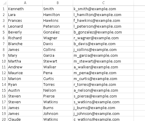
Figure 65-1:
Flash Fill can quickly convert these names into e-mail addresses.

It took only two examples before Flash Fill recognized the pattern and filled in the rest of the column.

Flash Fill is simpler than composing this equivalent formula:

=LOWER(LEFT(A1,1)&”_”&B1&”@example.com”)


Figure 65-2 shows another example. Column A:D hold the original data, and the text in column E was filled in using Flash Fill, after providing two examples. The equivalent formula to generate the text in column E is

=A4&” “&B4&”: “&TEXT(D4,”$0”)&” due on 10/”&C4&”/2013”


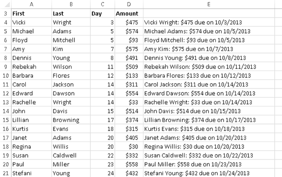
Figure 65-2:
Flash Fill generated the text in column E.

Tip 66: Inserting Stock Information

This tip describes how to insert refreshable stock data into a worksheet. For some reason, Microsoft makes this feature rather difficult to find.

Here’s how to do it:

1.
Make sure that you’re connected to the Internet.

2.
Type a stock symbol into a cell — for example,
MSFT
for Microsoft. Make sure the characters are all uppercase.

3.
Right-click the cell and choose Addition Cell Actions⇒Insert Refreshable Stock Price from the shortcut menu.

The Insert Stock Price dialog box appears.

4.
Specify the location for the information (on a new sheet, or starting at a particular cell).

5.
Click OK.

Excel retrieves current information about the stock and inserts data that occupies 18 rows and 16 columns (see Figure 66-1).

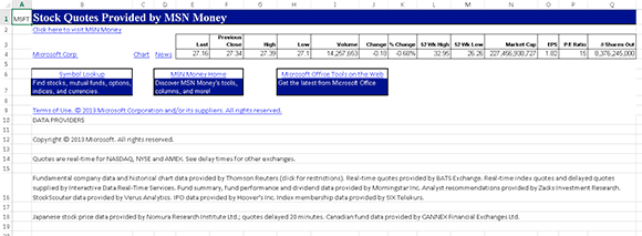
Figure 66-1:
Refreshable stock information inserted into a worksheet.

You can refresh the information at any time. Select any cell in the table, right-click, and choose Refresh from the shortcut menu. If your worksheet has information for multiple stocks, you can refresh them all by choosing Data⇒Connections⇒Refresh All.

Hiding irrelevant rows and columns

Notice that, of the 18 rows, only one of them contains actual data. The other rows are links and disclaimers. Unfortunately, there is no direct way to retrieve the information without all of the extraneous information. But you can hide the irrelevant rows and columns — and the hidden rows and columns remain hidden when you refresh the information.

Figure 66-2 shows a worksheet that has information for four stocks. I hid the irrelevant rows and columns, for a concise display.

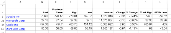
Figure 66-2:
Information for four stocks, after hiding irrelevant rows and columns.

Behind the scenes

Using the Addition Cell Actions⇒Insert Refreshable Stock Price shortcut menu item is just a quick way of performing a web query and retrieving data from Microsoft’s MSN Money site. You can retrieve the same information by performing a web query. Choose Data⇒Get External Data⇒From Web and use this URL:

http://moneycentral.msn.com/investor/external/excel/quotes.asp?symbol=MSFT


The URL retrieves information for Microsoft. You can replace MSFT with a different stock symbol. Figure 66-3 shows the New Web Query dialog box before the information is inserted into a worksheet.

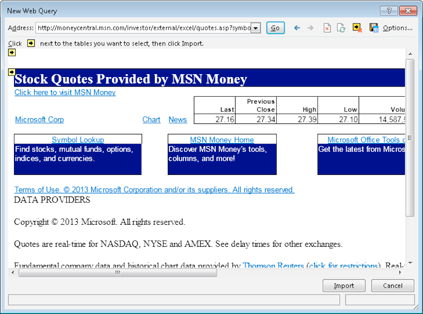
Figure 66-3:
Using the New Web Query dialog box to retrieve stock information.

  See Tip 67 for more information about web queries.

Tip 67: Getting Data from a Web Page

This tip describes three ways to capture data contained on a web page:

→ Paste a static copy of the information.

→ Create a refreshable link to the site.

→ Open the page directly in Excel.

Pasting static information

One way to get data from a web page into a worksheet is to simply highlight the text in your browser, press Ctrl+C to copy it to the Clipboard, and then paste it into a worksheet. The results will vary, depending on what browser you use and how the web page is coded.

If pasting doesn’t yield the results you want, choose Home⇒Clipboard⇒Paste⇒Paste Special and then try various paste options.

Figure 67-1 shows some currency exchange rates, pasted from a web page at msn.com. As you can see, even the hyperlinks are pasted.

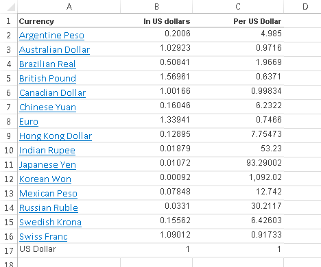
Figure 67-1:
A table of exchange rates copied from a website and pasted to a worksheet.

Pasting refreshable information

If you need to regularly access updated data from a web page, create a web query. Figure 67-1 shows a website that contains currency exchange rates in a three-column table.

The term web query is a bit misleading because this operation is not limited to the web. You can perform a web query on a local HTML file, a file stored on a network server, or a file stored on a web server on the Internet. To retrieve information from a web server, you must be connected to the Internet. After the information is retrieved, an Internet connection is not required to work with the information (unless you need to refresh the query).

These steps create a web query that allows this information to be retrieved and then refreshed at any time with a single mouse click:

1.
Choose Data⇒Get External Data⇒From Web to display the New Web Query dialog box.

2.
In the Address field, enter the URL of the website and click Go.

For this example, the URL for the web page shown in Figure 67-2 is