101 Excel 2013 Tips, Tricks and Timesavers (27 page)

http://investing.money.msn.com/investments/exchange-rates

Notice that the New Web Query dialog box contains a web browser (Internet Explorer). You can click links and navigate the website until you locate the data you’re interested in.

When a web page is displayed in the New Web Query dialog box, you see one or more yellow boxes with an arrow, which correspond to tables defined in the web page — plus another yellow box that will retrieve the entire page.

3.
Click a yellow box, and it turns into a green check box, which indicates that the data in that table will be imported.

Unfortunately, the table in the example is not selectable, so the only choice is to retrieve the entire page.

4.
Click the Import button to display the Import Data dialog box.

5.
In the Import Data dialog box, specify the location for the imported data.

It can be a cell in an existing worksheet or a new worksheet.

6.
Click OK, and Excel imports the data.

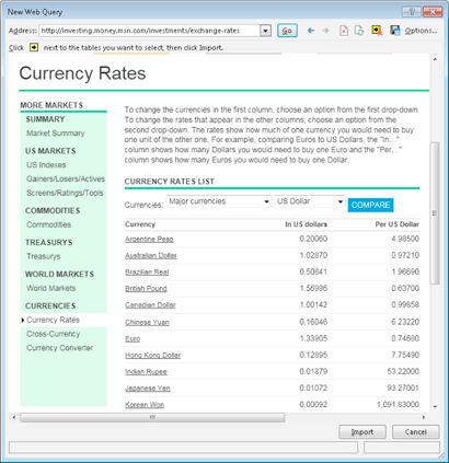
Figure 67-2:
Using the New Web Query dialog box to specify the data to be imported.

Part of the results is shown in Figure 67-3. Although I was interested only in the 17-row and 3-column currency table, this web query retrieved 145 rows of mostly irrelevant information.

By default, the imported data is a web query. To refresh the information, right-click any cell in the imported range and choose Refresh from the shortcut menu.

If you don’t want to create a refreshable query, specify this choice in Step 5 of the preceding step list. In the Import Data dialog box, click the Properties button and deselect the Save Query Definition check box.

Excel’s Web query feature works by identifying tables (specified using the HTML

tag) in the document. Increasingly, website designers use cascading style sheets (CSS) to display tabular information. As demonstrated in this example, Excel doesn’t recognize these as tables and, therefore, doesn’t display a yellow arrow so you can retrieve only the table. Therefore, you may have to retrieve the entire document and then delete (or hide) everything except the table that you want.

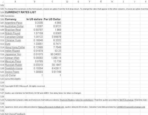
Figure 67-3:
Information retrieved from a web query.

Opening the web page directly

Another way to get web page data into a worksheet is to open the URL directly, by using Excel’s File⇒Open command. Just enter the complete URL into the File Name field and click Open.

The results will vary, depending on how the web page is laid out. Most of the time, you’ll get satisfactory results. In some cases, you’ll retrieve quite a bit of extraneous information. Also, note that the information is not refreshable. If the data on the web page changes, you’ll need to close the workbook and use the File⇒Open command again.

Tip 68: Importing a Text File into a Worksheet Range

If you need to insert a text file into a specific range in a worksheet, you may think that your only choice is to import the text into a new workbook (by choosing Office⇒Open) and then to copy the data and paste it to the range where you want it to appear. However, you can do it in a more direct way.

Figure 68-1 shows a small CSV (
c
omma
s
eparated
v
alue) file. The following instructions describe how to import this file, named monthly.csv, beginning at cell C3.

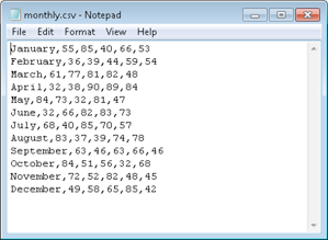
Figure 68-1:
This CSV file will be imported into a range.

1.
Choose Data⇒Get External Data⇒From Text to display the Import Text File dialog box.

2.
Navigate to the folder that contains the text file.

3.
Select the file from the list and then click the Import button to display the Text Import Wizard.

4.
Use the Text Import Wizard to specify how the data will be imported.

For a CSV file, specify Delimited, with a Comma Delimiter.

5.
Click the Finish button.

The Import Data dialog box appears.

6.
Click the Properties button, and the External Data Range Properties dialog box appears.

7.
Deselect the Save Query Definition check box and click OK to return to the Import Data dialog box.

8.
Here, specify the location for the imported data.

It can be a cell in an existing worksheet or a new worksheet.

9.
Click OK, and Excel imports the data (see Figure 68-2).

You can ignore Step 7 if the data you’re importing will be changing. By saving the query definition, you can quickly update the imported data by right-clicking any cell in the range and choosing Refresh.

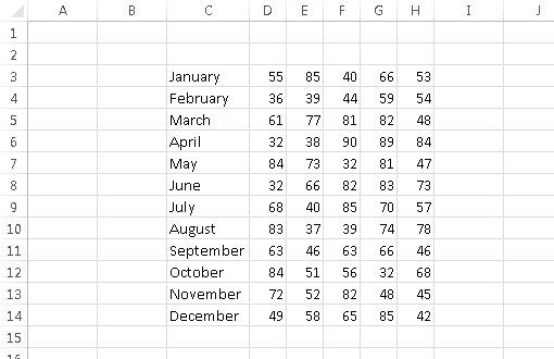
Figure 68-2:
This range contains data imported directly from a CSV file.

Tip 69: Using the Quick Analysis Feature

One of the new features in Excel 2013 is Quick Analysis. When you select a range of data, Excel displays a Quick Analysis button in the lower-right corner of the range. Click the button to view some options, shown in Figure 69-1. You can also press Ctrl+Q on the keyboard to display the Quick Analysis options.

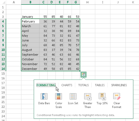
Figure 69-1:
Quick Analysis options for the selected range.

The words along the top (Formatting, Charts, Totals, Tables, and Sparklines) are menu items. Click an item and a different set of icons appears. When you hover your mouse over an icon, Excel sometimes displays a preview of how the option will appear.

The options available depend on the type of data in the selected range. For example, if the range contains only text, the Sparklines option will not be available.

Figure 69-2 shows an example of a range of numbers in column C, with a preview of the Quick Analysis option to create running totals in column D.

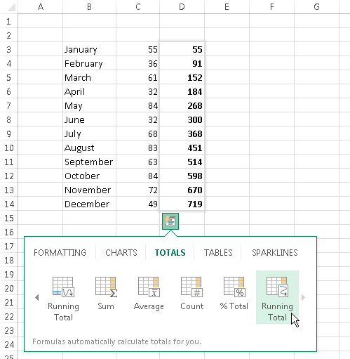
Figure 69-2:
A preview of Quick Analysis running totals.

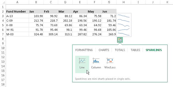
Figure 69-3 shows another example. The range A2:G7 is selected, and Quick Analysis is previewing the Line Sparklines option in column H.