101 Excel 2013 Tips, Tricks and Timesavers (22 page)

Figure 54-2:
Use the Auto Fill Options drop-down list to change the type of fill.

Here’s another AutoFill trick: If the data you start with is irregular, Excel completes the AutoFill action by doing a linear regression and fills in the predicted values. Figure 54-3 shows a worksheet with monthly sales values for January through July. If you use AutoFill after selecting C2:C8, Excel extends the best-fit linear sales trend and fills in the missing values. Figure 54-4 shows the predicted values, along with a chart.

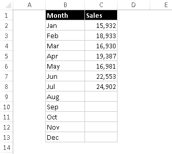
Figure 54-3:
Use AutoFill to perform a linear regression and predict sales values for August through December.

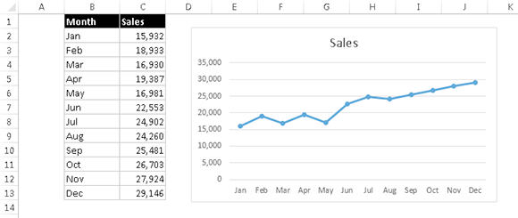
Figure 54-4:
The sales figures, after using AutoFill to predict the next five months.

AutoFill also works with dates and even a few text items — day names and month names. The following table lists a few examples of the types of data that can be autofilled.

You can also create your own lists of items to be autofilled. To do so, open the Excel Options dialog box and click the Advanced tab. Then scroll down and click the Edit Custom Lists button to display the Custom Lists dialog box. Enter your items in the List Entries box (each on a new line). Then click the Add button to create the list. Figure 54-5 shows a custom list of region names that use Roman numerals.

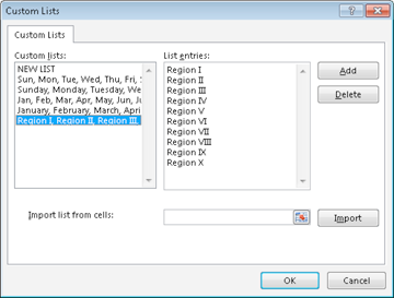
Figure 54-5:
These region names work with the Excel AutoFill feature.

Tip 55: Fixing Trailing Minus Signs

Imported data sometimes displays negative values with a trailing minus sign. For example, a negative value may appear as
3,498-
rather than the more common
-3,498
. Excel doesn’t convert these values. In fact, it considers them to be non-numeric text.

The solution is so simple it may surprise you:

1.
Select the data that has the trailing minus signs. The selection can also include positive values.

2.
Choose Data⇒Data Tools⇒Text to Columns.

3.
When the Text to Columns dialog box appears, click Finish.

This procedure works because of a default setting in the Advanced Text Import Settings dialog box (which you don’t even see, normally). To display this dialog box, shown in Figure 55-1, go to Step 3 in the Text to Columns Wizard dialog box and click Advanced.

Or you can use Flash Fill to fix the trailing minus signs. If the range contains any positive values, you may need to provide several examples. See Tip 64 for information about the Flash Fill feature.

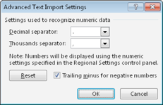
Figure 55-1:
The Trailing Minus for Negative Numbers option makes it very easy to fix trailing minus signs in a range of data.

Tip 56: Restricting Cursor Movement to Input Cells

A common type of worksheet uses two types of cells: input cells and formula cells. The user enters data into the input cells, and the formulas calculate and display the results.

Figure 56-1 shows a simple example. The input cells are in the range C4:C7. These cells are used by the formulas in C10:C13. To prevent the user from accidentally typing over formula cells, it’s useful to limit the cursor movement so that the formula cells can’t even be selected.

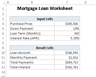
Figure 56-1:
This worksheet has input cells at the top and formula cells below.

Setting up this sort of arrangement is a two-step process: Unlock the input cells and then protect the sheet. The following specific instructions are for the example shown in Figure 56-1:

1.
Select C4:C7.

2.
Press Ctrl+1 to display the Format Cells dialog box.

3.
In the Format Cells dialog box, click the Protection tab, deselect the Locked check box, and click OK.

By default, all cells are locked.

4.
Choose Review⇒Changes⇒Protect Sheet.

The Protect Sheet dialog box appears.

5.
Deselect the Select Locked Cells check box and make sure that the Select Unlocked Cells check box is selected.

6.
(Optional) Specify a password that will be required to unprotect the sheet.

7.
Click OK.

After you perform these steps, only the unlocked cells can be selected. If you need to make any changes to your worksheet, you need to unprotect the sheet first, by choosing Review⇒Changes
➜
Unprotect Sheet.

Although this example used a contiguous range of cells for the input, that isn’t necessary for the steps to work. The input cells can be scattered throughout your worksheet.

Protecting a worksheet with a password isn’t a security feature. This type of password is easily cracked.

Tip 57: Transforming Data with and Without Using Formulas

Often, you have a range of cells containing data that must be transformed in some way. For example, you might want to increase all values by five percent. Or you might need to divide each value by two. This tip describes two ways to perform these types of transformations.

Transforming data without formulas

The following steps assume that you have values in a range and you want to increase all values by five percent. For example, the range can contain a price list and you’re raising all prices by five percent:

1.
Activate any empty cell and enter
1.05
.

You will multiply the values by this number, which results in an increase of five percent.

2.
Press Ctrl+C to copy that cell.

3.
Select the range to be transformed.

The range can include values, formulas, or text.

4.
Choose Home⇒Clipboard⇒Paste⇒Paste Special to display the Paste Special dialog box (see Figure 57-1).

5.
In the Paste Special dialog box, click the Multiply option.

6.
Click OK.

7.
Press Esc to cancel Copy mode.

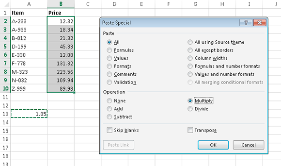
Figure 57-1:
Using the Paste Special dialog box to multiply a range by a value.

The values in the range are multiplied by the copied value (1.05), and cells that contain text are ignored. Formulas in the range are modified accordingly. Assume that the range originally contained this formula:

=SUM(B18:B22)


After you perform the Paste Special operation, the formula is converted to

=(SUM(B18:B22))*1.05


This technique is limited to the four basic math operations: add, subtract, multiply, and divide.

For more versatility, keep reading to learn how to use formulas to transform values.

Transforming data by using temporary formulas