101 Excel 2013 Tips, Tricks and Timesavers (12 page)
Read 101 Excel 2013 Tips, Tricks and Timesavers Online
Authors: John Walkenbach

Figure 24-2:
Using Registry Editor to add a new value to the Windows registry.
When you restart Excel, you’ll find that Excel no longer uses font substitution for small fonts. When font substitution is disabled, small text will be a bit more difficult to read, but the numbers will continue to line up, and you won’t see the #### display when you zoom out.
Figure 24-3 shows the worksheet in Figure 24-1, after disabling font substitution.
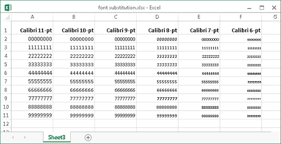
Figure 24-3:
Various font sizes, with font substitution disabled.
Tip 25: Updating Old Fonts
When you install Microsoft Office, several new fonts are added to your system, and these new fonts are used when you create a new workbook. The exact fonts that are used as defaults vary, depending on which document theme is in effect.
 See Tip 10 for more information about using document themes.
If you use the default Office theme, a newly created Excel workbook uses two new fonts: Cambria (for headings) and Calibri (for body text). When you open a workbook that was saved in a version prior to Excel 2007, the old fonts (probably Arial) aren’t updated. The difference in appearance between a worksheet that uses the old fonts and a worksheet that uses the new fonts is dramatic. When you compare an Excel 2003 worksheet with an Excel 2013 worksheet, the latter is much more readable and appears less cramped.
Figure 25-1 shows a workbook that was created in Excel 2003.
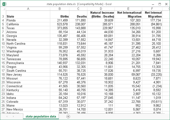
Figure 25-1:
This Excel 2003 workbook uses Arial 10-point font as the normal font.
To update the fonts in a workbook that was created in a previous version of Excel, follow these steps:
1.
Press Ctrl+N to create a new, blank workbook.
2.
Activate the workbook that uses the fonts to be updated.
3.
Choose Home⇒Styles⇒Merge Styles
The Merge Styles dialog box appears.
4.
In the Merge Styles dialog box, select the workbook that you created in Step 1 and click OK.
Excel asks whether you want to merge styles that have the same names.
5.
Reply by clicking the Yes button.
This procedure updates the fonts used in all cells except those that have additional formatting, such as a different font size, bold, italic, colored text, or a shaded background. To change the font in these cells, follow these steps:
1.
Select any single cell.
2.
Choose Home⇒Editing⇒Find & Select⇒Replace, or press Ctrl+H.
The Find and Replace dialog box appears.
3.
Make sure that the two Format buttons are visible. If these buttons aren’t visible, click the Options button to expand the dialog box.
4.
Click the upper Format button to display the Find Format dialog box.
5.
Click the Font tab.
6.
In the Font list, select the name of the font that you’re replacing (probably Arial, the old default font) and then click OK to close the Find Format dialog box.
7.
Click the lower Format button to display the Replace Format dialog box.
8.
Click the Font tab.
9.
In the Font list, select the name of the font that will replace the old font (probably Calibri) and then click OK to close the Replace Format dialog box.
10.
In the Find and Replace dialog box, click Replace All to replace the old font with the new font.
Figure 25-2 shows the Excel 2003 workbook after updating the font.
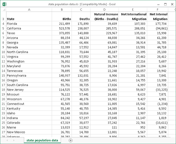
Figure 25-2:
This Excel workbook uses Calibri 11-point font as the normal font.
Part III: Formulas
The ability to create formulas is what makes a spreadsheet. In this part, you’ll find formula-related tips that can make your workbooks more powerful than ever.
Tips and Where to Find Them
Tip 26:
Resizing the Formula Bar
Tip 27:
Monitoring Formula Cells from Any Location
Tip 28:
Learning Some AutoSum Tricks
Tip 29:
Knowing When to Use Absolute and Mixed References
Tip 30:
Avoiding Error Displays in Formulas
Tip 31:
Creating Worksheet-Level Names
Tip 33:
Sending Personalized E-Mail from Excel
Tip 34:
Looking Up an Exact Value
Tip 35:
Performing a Two-Way Lookup
Tip 36:
Performing a Two-Column Lookup
Tip 38:
Calculating a Person’s Age
Tip 39:
Working with Pre-1900 Dates
Tip 40:
Displaying a Live Calendar in a Range
Tip 41:
Returning the Last Nonblank Cell in a Column or Row
Tip 42:
Various Methods of Rounding Numbers
Tip 43:
Converting Between Measurement Systems
Tip 44:
Counting Nonduplicated Entries in a Range
Tip 45:
Using the AGGREGATE Function
Tip 46:
Making an Exact Copy of a Range of Formulas
Tip 47:
Using the Background Error-Checking Features
Tip 48:
Using the Inquire Add-In
Tip 49:
Hiding and Locking Your Formulas
Tip 50:
Using the INDIRECT Function
Tip 26: Resizing the Formula Bar
In earlier versions of Excel, editing a cell that contains a lengthy formula or lots of text often obscures the worksheet. Figure 26-1 shows Excel 2003 when a cell that contains lengthy text is selected. Notice that many of the cells are covered up by the expanded Formula bar. Beginning with Excel 2007, this problem is corrected.
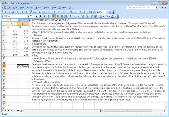
Figure 26-1:
In older versions of Excel, editing a lengthy formula or a cell that contains lots of text often obscures the worksheet.
The Excel 2013 Formula bar displays a small arrow on the right; click the arrow, and the Formula bar expands. You can also drag the bottom border of the Formula bar to change its height. Also useful is a shortcut key combination: Ctrl+Shift+U. Pressing this key combination toggles the height of the Formula bar to show either one row or the previous size. If the expanded Formula bar isn’t tall enough to display all of the text in the active cell, a scrollbar displays to the right of the Formula bar.
Figure 26-2 shows an example of the resized Formula bar. As you can see, increasing the height of the Formula bar doesn’t obscure the information in the worksheet. Instead, the worksheet information is displayed below the Formula bar. You can make the formula bar almost as tall as the workbook window (one worksheet row always remains visible).
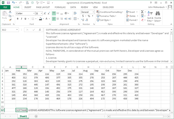
Figure 26-2:
Changing the height of the formula bar makes it much easier to edit lengthy formulas and text, and you can still view all cells in your worksheet.
You can also resize the width of the Formula bar. Click and drag the three dots to the right of the Name box. When the Name box gets wider, the Formula bar gets narrower.
Tip 27: Monitoring Formula Cells from Any Location
If you have a large spreadsheet model, you might find it helpful to monitor the values in a few key cells as you change various input cells. The Watch Window feature makes this task very simple. Using the Watch Window, you can keep an eye on any number of cells, regardless of which worksheet or workbook is active. Using this feature can save time and eliminate scrolling and switching among worksheet tabs and workbook windows.
About the Watch Window
To display the Watch Window, choose Formulas⇒Formula Auditing⇒Watch Window. To watch a cell, click the Add Watch button in the Watch Window and then specify the cell in the Add Watch dialog box. When the Add Watch dialog box opens, you can add multiple cells by selecting a range or by pressing Ctrl and clicking individual cells.
For each cell, the Watch Window displays the workbook name, the worksheet name, the cell name (if it has one), the cell address, the current value, and the formula (if it has one).
Excel remembers the cells in a Watch Window, even between sessions. If you close a workbook that contains cells being monitored in the Watch Window, those cells are removed from the Watch Window. But if you reopen that workbook, the cells are displayed again.
Figure 27-1 shows the Watch Window, with several cells being monitored.
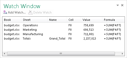
Figure 27-1:
Using the Watch Window to monitor the value of formula cells.
Customizing the Watch Window
The Watch Window is a task pane, and you can customize the display by doing any of the following:
→ Click and drag a border to change the size of the task pane.
→ Drag the task pane to an edge of an Excel workbook window, and it becomes docked rather than free floating.
→ Click and drag the borders in the header to change the width of the columns displayed. By dragging a column border all the way to the left, you can hide the column.
→ Click one of the headers to sort the contents by that column.
Navigating with the Watch Window
You can also use the Watch Window as a navigational aid. If you find that you often need to switch among worksheets, add a cell for each worksheet to the Watch Window. To activate a cell displayed in the Watch Window, double-click it in the Watch Window.
 Unfortunately, in Excel 2013, this navigational technique works only with the active workbook. In other words, double-clicking a Watch Window item that points to a cell in a different workbook will not activate the workbook. I don’t know if this is by design or if it’s a bug in Excel 2013.
Tip 28: Learning Some AutoSum Tricks
Just about every Excel user knows about the AutoSum button. This command is so popular that it’s available in two Ribbon locations: in the Home⇒Editing group and in the Formulas⇒Function Library group.
Just activate a cell and click the button, and Excel analyzes the data surrounding the active cell and proposes a SUM formula. If the proposed range is correct, click the AutoSum button again (or press Enter), and the formula is inserted. If you change your mind, press Esc.
Be careful if the range to be summed contains any blank cells. A blank cell will cause Excel to misidentify the complete range. If Excel incorrectly guesses the range to be summed, just select the correct range to be summed and press Enter.
You can also access AutoSum using your keyboard. Pressing Alt+= has exactly the same effect as clicking the AutoSum button.
The AutoSum button can insert other types of formulas. Notice the little arrow on the right side of that button? Click it, and you see four other functions: AVERAGE, COUNT, MAX, and MIN (see Figure 28-1). Click one of those items, and the appropriate formula is proposed. You also see a More Functions item, which simply displays the Insert Function dialog box — the same one that appears when you choose Formulas⇒Function Library⇒Insert Function (or click the fx button to the left of the formula bar).
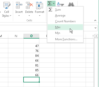
Figure 28-1:
Using the AutoSum button to insert other functions.
In some situations (described next), AutoSum creates formulas automatically and doesn’t give you an opportunity to review the range to be summed. Don’t assume that Excel guessed the range correctly.
Following are some additional tricks related to AutoSum:
→ If you need to enter a similar SUM formula into a range of cells, select the entire range before you click the AutoSum button. In this case, Excel inserts the functions for you without asking you — one formula in each of the selected cells.
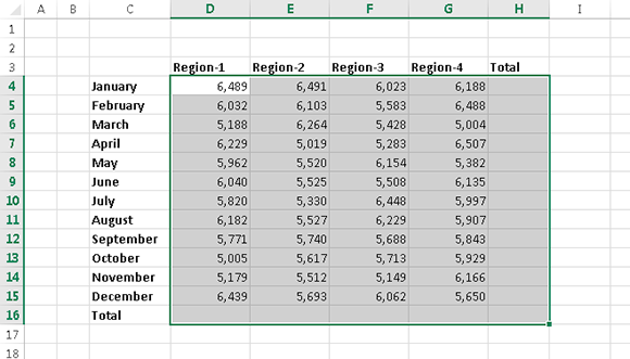
→ To sum both across and down a table of numbers, select the range of numbers plus an additional column to the right and an additional row at the bottom. Click the AutoSum button, and Excel inserts the formulas that add the rows and the columns. In Figure 28-2, the range to be summed is D4:G15, so I selected an additional row and column: D4:H16. Clicking the AutoSum buttons puts formulas in row 16 and column H.
→ If you’re working with a table (created by choosing Insert⇒Tables⇒Table), using the AutoSum button after selecting the row below the table inserts a Total row for the table and creates formulas that use the SUBTOTAL function rather than the SUM function. The SUBTOTAL function sums only the visible cells in the table, which is useful if you filter the data.
→ Unless you applied a different number format to the cell that will hold the SUM formula, AutoSum applies the same number format as the first cell in the range to be summed.
→ To create a SUM formula that uses only
some
of the values in a column, select the cells to be summed and then click the AutoSum button. Excel inserts the SUM formula in the first empty cell below the selected range. The selected range must be a contiguous group of cells — a multiple selection isn’t allowed.