101 Excel 2013 Tips, Tricks and Timesavers (17 page)

Figure 39-3:
Using custom functions to work with pre-1900 dates.

The extended date functions don’t make any adjustments for changes made to the calendar in 1582. Consequently, working with dates prior to October 15, 1582, may not yield correct results.

Use a different product

A final option is to use a different spreadsheet product that supports pre-1900 dates. Figure 39-4 shows Google Spreadsheet. This (free) product uses the same date serial number system as Excel, but uses negative values for dates prior to 1900. It supports dates from 1583 through 9956.

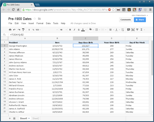
Figure 39-4:
Google Spreadsheet can handle pre-1900 dates.

Tip 40: Displaying a Live Calendar in a Range

This tip describes how to create a “live” calendar in a range of cells. Figure 40-1 shows an example. If you change the date that’s displayed at the top of the calendar, the calendar recalculates to display the dates for the month and year.

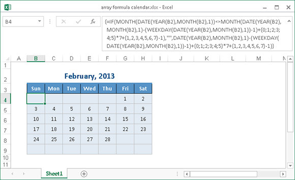
Figure 40-1:
This calendar was created with a complex array formula.

To create this calendar in the range B2:H9, follow these steps:

1.
Select B2:H2 and then merge the cells by choosing Home⇒Alignment⇒Merge & Center.

2.
Enter a date into the merged range.

The day of the month isn’t important, so change the format of the cell to a custom format that doesn’t display the day: mmmm, yyyy.

3.
Enter the abbreviated day names in the range B3:H3.

4.
Select B4:H9 and then enter the following array formula without the line breaks.

Note:
To enter an array formula, press Ctrl+Shift+Enter (not just Enter):

=IF(MONTH(DATE(YEAR(B2),MONTH(B2),1))

<>MONTH(DATE(YEAR(B2),MONTH(B2),1)-

(WEEKDAY(DATE(YEAR(B2),MONTH(B2),1))-1)

+{0;1;2;3;4;5}*7+{1,2,3,4,5,6,7}-1),””,

DATE(YEAR(B2),MONTH(B2),1)-

(WEEKDAY(DATE(YEAR(B2),MONTH(B2),1))-1)

+{0;1;2;3;4;5}*7+{1,2,3,4,5,6,7}-1)


5.
Select the range B4:H9 and choose Home⇒Number⇒More Number formats to display the Number tab of the Format Cells dialog box.

6.
In the Format Cells dialog box, choose Custom and enter the following custom number format (which displays the day only) in the Type field:

d

7.
Adjust the column widths and format the cells the way you like.

Change the date and year in cell B2, and the calendar updates automatically. After creating this calendar, you can copy the range to any other worksheet or workbook.

Tip 41: Returning the Last Nonblank Cell in a Column or Row

Suppose that you update a worksheet frequently by adding new data to its columns. You might need a way to reference the last value in a particular column (the value most recently entered). This tip presents three ways to accomplish this.

Figure 41-1 shows an example. The worksheet tracks the value of three funds in columns B:D. Notice that the information does not arrive at the same time. The goal is to get the sum of the most recent data for each fund. These values are calculated in the range G4:G6.

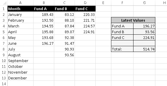
Figure 41-1:
Use a formula to return the last non-empty cell in columns B:D.

Cell counting method

The formulas in G4, G5, and G6 are

=INDEX(B:B,COUNTA(B:B))


=INDEX(C:C,COUNTA(C:C))


=INDEX(D:D,COUNTA(D:D))


These formulas use the COUNTA function to count the number of non-empty cells in column C. This value is used as the second argument for the INDEX function. For example, in column B the last value is in row 6, COUNTA returns 6, and the INDEX function returns the 6th value in the column.

The preceding formulas work in most, but not all, situations. If the column has one or more empty cells interspersed, determining the last nonblank cell is a bit more challenging because the COUNTA function doesn’t count the empty cells.

Array formula method

The following array formula returns the contents of the last non-empty cell in the first 500 rows of column B, even if column B contains blank cells:

=INDEX(B:B,MAX(ROW(B:B)*(B:B<>””)))


Press Ctrl+Shift+Enter (not just Enter) to enter an array formula.

You can, of course, modify the formula to work with a column other than column B. To use a different column, change the four column references from B to whatever column you need.

You can’t use this formula, as written, in the same column in which it’s working. Attempting to do so generates a circular reference. You can, however, modify it. For example, to use the function in cell B1, change the references so that they begin with row 2 rather than the entire columns. For example, use B2:B1000 to return the last non-empty cell in the range B2:B1000.

The following array formula is similar to the previous formula, but it returns the last non-empty cell in a row (in this case, row 1):

=INDEX(1:1,MAX(COLUMN(1:1)*(1:1<>””)))


To use this formula for a different row, change the three 1:1 row references to correspond to the correct row number.

Standard formula method

The final method uses a standard (non-array) formula, and is rather cryptic. This formula returns the last non-empty cell in column B:

=LOOKUP(2,1/(B:B<>””),B:B)


This formula ignores error values, so if the last non-empty cell contains an error (such as #DIV/0!), the formula returns the last non-empty, non-error cell.

The following formula returns the last non-empty, non-error cell in row 1:

=LOOKUP(2,1/(1:1<>””),1:1)


Tip 42: Various Methods of Rounding Numbers

Rounding numbers is a common task, and Excel provides quite a few functions that round values in various ways.

You must understand the difference between
rounding
a value and
formatting
a value. When you
format
a number to display a specific number of decimal places, formulas that refer to that number use the actual value, which might differ from the displayed value. When you
round
a number, formulas that refer to that value use the rounded number.

Table 42-1 summarizes the Excel rounding functions.

Table 42-1:
Excel Rounding Functions

The following sections provide examples of formulas that use various types of rounding.

Rounding to the nearest multiple

The MROUND function is useful for rounding values to the nearest multiple. For example, you can use this function to round a number to the nearest 5. The following formula returns 135:

=MROUND(133,5)


Rounding currency values

Often, you need to round currency values. For example, a calculated price might be a number like $45.78923. In such a case, you want to round the calculated price to the nearest penny. This process might sound simple, but you can round this type of value in one of three ways:

→ Round it up to the nearest penny.

→ Round it down to the nearest penny.

→ Round it to the nearest penny (the rounding can be up or down).

The following formula assumes that a dollar-and-cents value is in cell A1. The formula rounds the value to the nearest penny. For example, if cell A1 contains $12.421, the formula returns $12.42.

=ROUND(A1,2)


If you need to round up the value to the nearest penny, use the CEILING.MATH function. The following formula rounds up the value in cell A1 to the nearest penny (if, for example, cell A1 contains $12.421, the formula returns $12.43):