101 Excel 2013 Tips, Tricks and Timesavers (7 page)
Read 101 Excel 2013 Tips, Tricks and Timesavers Online
Authors: John Walkenbach

Besides Excel 2013, three other versions of Excel for Windows are still widely used: Excel 2003, Excel 2007, and Excel 2010.
If you create workbooks only for Excel 2013 users, you can skip this tip because you don’t have to be concerned with compatibility. But if you create workbooks for those who use an earlier version, you need to understand compatibility.
The Excel 2013 file formats
The current Excel file formats (all of which were introduced in Excel 2007) are
→ .xlsx: A workbook file that doesn’t contain macros
→ .xlsm: A workbook file that contains macros
→ .xltx: A workbook template file that doesn’t contain macros
→ .xltm: A workbook template file that contains macros
→ .xlsa: An add-in file
→ .xlsb: A binary file that’s similar to the old .xls format but able to accommodate the new features
→ .xlsk: A backup file
With the exception of .xlsb, these are all “open” XML files, which means that the file format is not proprietary and other applications can read and write these types of files.
 The XML files are actually zip-compressed text files. If you rename one of these files to have a .zip extension, you can examine the contents using any of several zip file utilities — including the zip file support built into Windows. Taking a look at the innards of an Excel workbook is an interesting exercise for curious-minded users.
The Office Compatibility Pack
Normally, those who use a version prior to Excel 2007 can’t open workbooks saved in the newer Excel file formats. But, fortunately, Microsoft has released a free Compatibility Pack for Office 2003 and Office XP.
If an Office 2003 or Office XP user installs the Compatibility Pack, he can open files created in Office 2007 or later and save files in the newer format. The Office programs that are affected are Excel, Word, and PowerPoint. This software doesn’t endow the older versions with any new features — it just gives them the capability to open and save files in the new format.
To download the Compatibility Pack from Microsoft, search the web for
Office Compatibility Pack.
It’s important to understand the limitations regarding version compatibility. Even though your colleague is able to open your file, there is no guarantee that everything will function correctly or look the same.
Checking compatibility
If you save your workbook to an older file format (such as .xls, for versions prior to Excel 2007), Excel automatically runs the Compatibility Checker. The Compatibility Checker identifies the elements of your workbook that will result in a loss of functionality or fidelity (cosmetics).
Figure 11-1 shows the Compatibility Checker dialog box. Click the Select Versions to Show button to limit the compatibility-checking to a specific version of Excel.
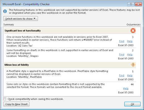
Figure 11-1:
The Compatibility Checker is a useful tool for those who share workbooks with other people.
The bottom part of the Compatibility Checker lists the potential compatibility problems. To display the results in a more readable format, click the Copy to New Sheet button.
Keep in mind that compatibility problems also can occur with Excel 2007 and Excel 2010, even though these versions use the same file format as Excel 2013. You can’t expect features that are new to Excel 2013 to work in earlier versions. For example, if you add slicers to table (a new feature in Excel 2013) and send it to a colleague who uses Excel 2010, the slicers won’t be displayed. In addition, formulas that use any of the new worksheet functions will return an error. The Compatibility Checker identifies these types of problems.
Tip 12: Where to Change Printer Settings
If you want to print a copy of a worksheet with no fuss and bother, use the Quick Print option. One way to access this command is to choose File⇒Print (which displays the Print pane of Backstage view) and then click the Print button.
However, if the default print settings aren’t good enough, you must make some adjustments. A little tweaking of the print settings can often improve your printed reports.
Unfortunately, Excel has no one-stop location for adjusting print setting. You can adjust print settings in three places:
→ The Print settings screen in Backstage view, which opens when you choose File⇒Print.
→ The Page Layout tab of the Ribbon.
→ The Page Setup dialog box, which opens when you click the dialog launcher in the lower-right corner of the Page Layout⇒Page Setup group on the Ribbon. You can also access the Page Setup dialog box from the Print settings screen in Backstage view.
Table 12-1 summarizes the locations where you can make various types of print-related adjustments in Excel 2013.
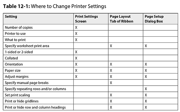
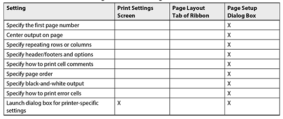
This table might make printing seem more complicated than it really is. The key point to remember is this: If you can’t find a way to make a particular adjustment, it’s probably available from the Page Setup dialog box.
Part II: Formatting
Excel has lots of formatting options to make your work look good. In this part, you’ll find tips that cover formatting numbers, copying formatting, and other topics.
Tips and Where to Find Them
Tip 13:
Working with Merged Cells 43
Tip 14:
Indenting Cell Contents 48
Tip 16:
Creating Custom Number Formats 54
Tip 17:
Using Custom Number Formats to Scale Values 58
Tip 18:
Creating a Bulleted List 60
Tip 19:
Shading Alternate Rows Using Conditional Formatting 62
Tip 20:
Formatting Individual Characters in a Cell 65
Tip 21:
Using the Format Painter 66
Tip 22:
Inserting a Watermark 68
Tip 23:
Showing Text and a Value in a Cell 70
Tip 13: Working with Merged Cells
Merging cells is a simple concept: Join two or more cells to create a larger single cell. To merge cells, just select them and choose Home⇒Alignment⇒Merge & Center. Excel combines the selected cells and displays the contents of the upper-left cell, centered.
Merging cells is usually done as a way to enhance the appearance of a worksheet. Figure 13-1, for example, shows a worksheet with four sets of merged cells: C2:I2, J2:P2, B4:B8, and B9:B13. The merged cells in column B also use vertical text.
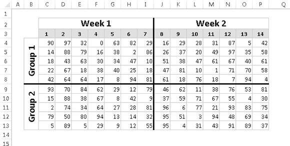
Figure 13-1:
This worksheet has four sets of merged cells.
Remember that merged cells can contain only one piece of information: a single value, text, or a formula. If you attempt to merge a range of cells that contains more than one nonempty cell, Excel prompts you with a warning that only the data in the upper-leftmost cell will be retained.
To unmerge cells, just select the merged area and click the Merge and Center button again.
Other merge actions
Notice that the Merge and Center button is a drop-down menu. If you click the arrow, you see three additional commands:
→
Merge Across:
Lets you select a range and then creates multiple merged cells — one for each row in the selection.
→
Merge Cells:
Works just like Merge and Center, except that the content of the upper-left cell is not centered. (It retains its original horizontal alignment.)
→
Unmerge Cells:
Unmerges the selected merged cell.
Wrapping text in merged cells is an easy way to display lengthy text. To make text wrap in merged cells, select the merged cells and choose Home⇒Alignment⇒Wrap Text. Use the vertical and horizontal alignment controls in Home⇒Alignment group to adjust the text position.
Figure 13-2 shows a worksheet in which 171 cells have been merged (19 rows and 9 columns). The text in the merged cells uses the Wrap Text option.

Figure 13-2:
Here 171 cells are merged into one.
Potential problems with merged cells
Many Excel users have a deep-seated hatred of merged cells. They avoid using this feature and urge everyone else to also avoid merged cells. But if you understand the limitations and potential problems, there’s no reason to completely avoid using merged cells.
Here are a few things to keep in mind:
→ You can’t use merged cells in a table (created by choosing Insert⇒Tables⇒Table). This is understandable because data in a table must be consistent in terms of rows and columns. Merging cells in a table will destroy that consistency.
→ Normally, you can double-click a column header or row header to autofit the data in the column or row, but that feature doesn’t work if the row or column contains merged cells. Instead, you need to adjust the column width or row height manually.
→ Merged cells can also affect sorting and filtering. That’s another reason why merged cells aren’t allowed in tables. If you have a range of data that you will sort or filter, avoid using merged cells.
→ Finally, merged cells can cause problems with VBA macros. For example, if the cells in A1:D1 are merged, a VBA statement such as the following will actually select four columns (not at all what the programmer intended):
Columns(“B:B”).Select
Locating all merged cells
To find out whether a worksheet contains merged cells, follow these steps:
1.
Press Ctrl+F to open the Find and Replace dialog box.
2.
Check to be sure the Find What field is empty.
3.
Click the Options button to expand the dialog box.
4.
Click the Format button to open the Find Format dialog box, where you specify the formatting to find.
5.
In the Find Format dialog box, choose the Alignment tab and place a check mark next to Merged Cells.
6.
Click OK to close the Find Format dialog box.
7.
In the Find and Replace dialog box, click Find All.
Excel displays a list of all merged cells in the worksheet (see Figure 13-3). Click an address in the list, and the merged cell is activated.
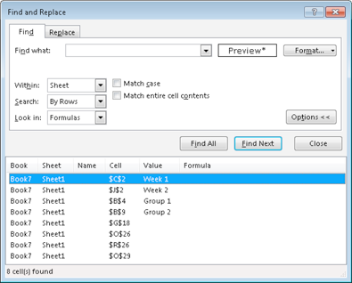
Figure 13-3:
Finding all merged cells in a worksheet.
Unmerging all merged cells
Here’s a quick way to unmerge all merged cells in a worksheet:
1.
Select all cells in the worksheet.
A quick way to do so is to click the triangle at the intersection of the row headers and column headers.
2.
Click the Home tab.
3.
If the Merge & Center command is highlighted, click it.
In Step 3, if the Merge & Center command isn’t highlighted, there are no merged cells. If you click the command when all cells are selected, all 17,179,869,184 cells in the worksheet will be merged.
Alternatives to merged cells
In some cases, you can use Excel’s Center Across Selection command as an alternative to merged cells. This command is useful for centering text across several columns.
1.
Enter the text to be centered in a cell.
2.
Select the cell that has the text and additional cells to the right of it.
3.
Press Ctrl+1 to display the Format Cells dialog box.
4.
In the Format Cells dialog box, choose the Alignment tab.
5.
In the Text Alignment section, choose the Horizontal drop-down and select Center Across Selection.
6.
Click OK to close the Format Cells dialog box.
The text is centered across the selected cells.
Another alternative to merging cells is to use a text box. This is particular useful for text that must be displayed vertically. Figure 13-4 shows an example of a text box that displays vertical text. To add a text box, choose Insert⇒Text⇒Text Box, draw the box on the worksheet, and then enter the text. Use the text formatting tools on the Home tab to adjust the text; use the tools in the Drawing Tools⇒Format context tab to make other modifications (for example, to hide the text box outline).
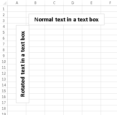
Figure 13-4:
Using a text box as an alternative to merged cells.
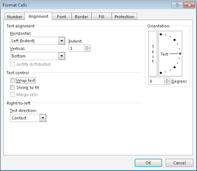
Tip 14: Indenting Cell Contents
As you probably know, Excel (by default) left-aligns text and right-aligns numbers. Most of the time, that’s exactly how you want data to be aligned.
But if a column of text is to the right of a column of numbers, the information can be difficult to read. Figure 14-1 shows an example. All the data in this table uses the default alignment. The table would be more legible if there were a larger gap between the numbers and the text.
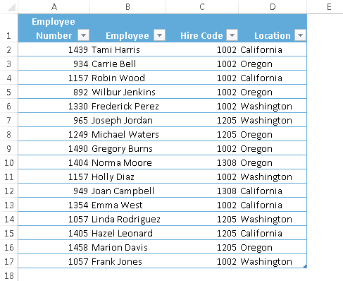
Figure 14-1:
The legibility of this table can be improved by indenting the text.
Many users don’t realize that Excel can indent data — either from the left or from the right. Unfortunately, the command to indent is not on the Ribbon. You need to select the cells and then use the Alignment tab of the Format Cells dialog box (see Figure 14-2). A quick way to access this dialog box is to click the dialog launcher icon in the lower-right corner of the Home⇒Alignment group.