101 Excel 2013 Tips, Tricks and Timesavers (15 page)
Read 101 Excel 2013 Tips, Tricks and Timesavers Online
Authors: John Walkenbach

Figure 33-2 shows how it looks when Windows Live Mail is the default e-mail client.
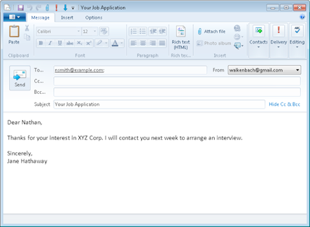
Figure 33-2:
This e-mail message was composed by the HYPERLINK function.
Tip 34: Looking Up an Exact Value
The VLOOKUP and HLOOKUP functions are useful if you need to return a value from a table (in a range) by looking up another value.
The classic example of a lookup formula involves an income tax rate schedule (see Figure 34-1). The tax rate schedule shows the income tax rates for various income levels. The following formula (in cell B3) returns the tax rate for the income value in cell B2:
=VLOOKUP(B2,D2:F7,3)
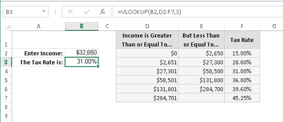
Figure 34-1:
Using VLOOKUP to look up a tax rate.
The tax table example demonstrates that VLOOKUP and HLOOKUP don’t require an exact match between the value to be looked up and the values in the lookup table. In some cases, though, you might require a perfect match. For example, when looking up an employee number, close doesn’t count. You require an exact match for the number.
To look up only an exact value, use the VLOOKUP (or HLOOKUP) function with the optional fourth argument set to FALSE.
Figure 34-2 shows a worksheet with a lookup table that contains employee numbers (column D) and employee names (column E). The formula in cell B2, which follows, looks up the employee number entered in cell B1 and returns the corresponding employee name:
=VLOOKUP(B1,D1:E11,2,FALSE)
Because the last argument for the VLOOKUP function is FALSE, the function returns a value only if an exact match is found. If the value isn’t found, the formula returns #N/A. This is exactly what you want to happen, of course, because returning an approximate match for an employee number makes no sense. Also, notice that the employee numbers in column D aren’t in ascending order. If the last argument for VLOOKUP is FALSE, the values don’t need to be in ascending order.
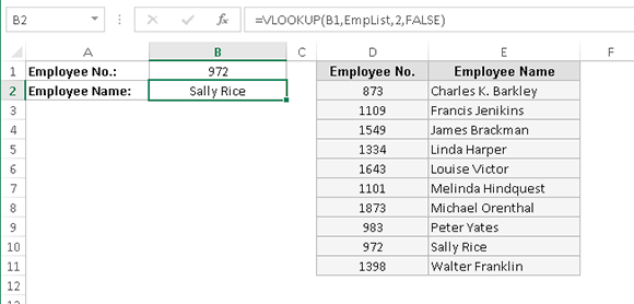
Figure 34-2:
This lookup table requires an exact match.
If you prefer to see something other than #N/A when the employee number isn’t found, you can use the IFERROR function to test for the #N/A result (using the ISNA function) and substitute a different string. The following formula displays the text “Not Found” rather than #N/A:
=IFERROR(VLOOKUP(B2,D1:E11,2,FALSE),”Not Found”)
The IFERROR function was introduced in Excel 2007, so if your workbook must be compatible with Excel 2003 and earlier versions, use this formula:
=IF(ISERROR(VLOOKUP(B2,D1:E11,2,FALSE)),”Not Found”,
VLOOKUP(B2,D1:E11,2,FALSE))
Tip 35: Performing a Two-Way Lookup
A two-way lookup identifies the value at the intersection of a column and a row. This tip describes two methods to perform a two-way lookup.
Using a formula
Figure 35-1 shows a worksheet with a range that displays product sales by month. To retrieve sales for a particular month and product, the user enters a month in cell B1 and a product name in cell B2.
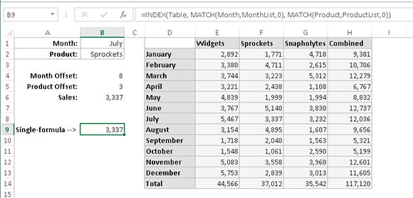
Figure 35-1:
This table demonstrates a two-way lookup.
To simplify the process, the worksheet uses the named ranges shown in the following minitable.
Name | Refers To |
Month | B1 |
Product | B2 |
Table | D1:H14 |
MonthList | D1:D14 |
ProductList | D1:H1 |
The following formula (in cell B4) uses the MATCH function to return the position of the Month within the MonthList range. For example, if the month is January, the formula returns 2 because January is the second item in the MonthList range (the first item is a blank cell, D1):
=MATCH(Month,MonthList,0)
The formula in cell B5 works similarly but uses the
ProductList
range:
=MATCH(Product,ProductList,0)
The final formula, in cell B6, returns the corresponding sales amount. It uses the INDEX function with the results from cells B4 and B5:
=INDEX(Table,B4,B5)
You can combine these formulas into a single formula, as shown here:
=INDEX(Table,MATCH(Month,MonthList,0),MATCH(Product,ProductList,0))
Using implicit intersection
The second method to accomplish a two-way lookup is quite a bit simpler, but it requires that you create a name for each row and column in the table.
A quick way to name each row and column is to select the table and choose Formulas⇒Defined Names⇒Create from Selection. In the Create Names from Selection dialog box, specify that the names are in the top row and left column (see Figure 35-2). Click OK, and Excel creates the names.
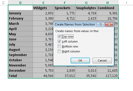
Figure 35-2:
Creating range names automatically.
After creating the names, you can use a simple formula to perform the two-way lookup, such as
=Sprockets July
This formula, which uses the range intersection operator (a space), returns July sales data for Sprockets.
Tip 36: Performing a Two-Column Lookup
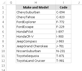
Some situations may require a lookup based on the values in two columns. Figure 36-1 shows an example.
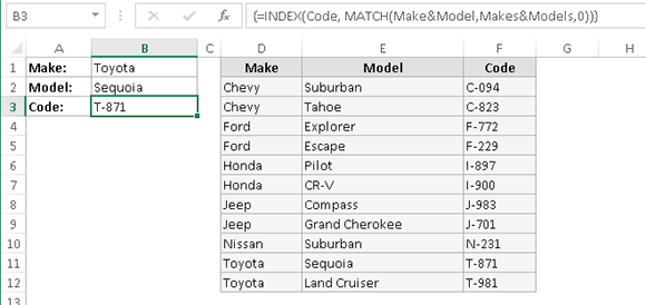
Figure 36-1:
This workbook performs a lookup by using information in two columns (D and E).
The lookup table contains automobile makes and models and a corresponding code for each one. The technique described here allows you to look up the value based on the car’s make and model.
The worksheet uses named ranges, as shown in the following minitable.
Range | Name |
F2:F12 | Code |
B1 | Make |
B2 | Model |
D2:D12 | Range1 |
E2:E12 | Range2 |
The following array formula displays the corresponding code for an automobile make and model:
=INDEX(Code,MATCH(Make&Model,Range1&Range2,0))
 When you enter an array formula, press Ctrl+Shift+Enter (not just Enter).
This formula works by concatenating the contents of Make and Model and then searching for this text in an array consisting of the corresponding concatenated text in
Range1
and
Range2
.
An alternative approach is to create a new two-column lookup table, as shown in Figure 36-2. This table contains the same information as the original table, but column H contains the data from columns D and E, concatenated.