101 Excel 2013 Tips, Tricks and Timesavers (19 page)
Read 101 Excel 2013 Tips, Tricks and Timesavers Online
Authors: John Walkenbach

Fortunately, Excel provides “formula autocomplete” assistance when you enter this function in a formula. Figure 45-1 shows the drop-down list of arguments that appears automatically. Choose the argument and press Tab to continue.
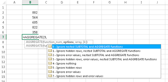
Figure 45-1:
Using autocomplete to identify the argument values for AGGREGATE.
Figure 45-2 shows an example of how the AGGREGATE function can be useful. The worksheet contains pre-test and post-scores for eight students. Note that Charles did not take the post-test, so cells C4 and D4 contain the NA/# error value (to indicate not available).
Cell D11 contains a formula that uses the AVERAGE function to calculate the average change. This formula returns an error:
=AVERAGE(D2:D9)
The formula in cell D12 uses the AGGREGATE function, with the option to ignore error values:
=AGGREGATE(1,6,D2:D9)
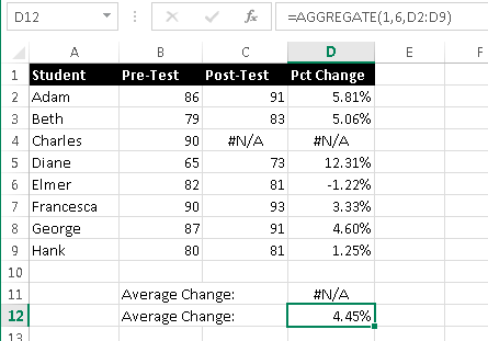
Figure 45-2:
Using the AGGREGATE function to calculate an average when the range contains an error value.
Remember that AGGREGATE works only with Excel 2010 and later. If a workbook that uses this function is opened in a previous version of Excel, the formula will display an error.
Tip 46: Making an Exact Copy of a Range of Formulas
When you copy a cell that contains a formula, Excel adjusts all the relative cell references. Assume that cell D1 contains this formula:
=A1*B1
When you copy this cell, the two cell references are changed relative to the destination. If you copy D1 to D12, for example, the copied formula is
=A12*B12
Sometimes, you may prefer to make an exact copy of a formula. One way is to convert all the cell references to absolute references (for example, change =A1*B1 to =$A$1*$B$1). Another way is to (temporarily) remove the equal sign from the formula, which converts the formula to text. Then you can copy the cell and manually insert the equal sign into the original formula and the copied formula.
What if you have a large range of formulas and you want to make an exact copy of those formulas? Editing each formula is tedious and error-prone. Here’s a way to accomplish the task. It uses Windows Notepad, but any text editor (including Microsoft Word) will do.
For the following steps, assume that you want to copy the formulas in A1:D10 on Sheet1 and make an exact copy in A13:D22, also on Sheet1:
1.
Put Excel in Formula view mode.
To toggle Formula view mode, choose Formulas⇒Formula Auditing⇒Show Formulas.
2.
Select the range to copy. In this case, A1:D10 on Sheet1.
3.
Press Ctrl+C to copy the range.
4.
Launch the Windows Notepad text editor.
5.
Press Ctrl+V to paste the copied data into Notepad.
6.
In Notepad, press Ctrl+A to select all of the text, followed by Ctrl+C to copy the text.
7.
Activate Excel and activate the upper-left cell where you want to paste the formulas (in this example, A13 on Sheet2) and make sure that the sheet you’re copying to is in Formula view mode.
8.
Press Ctrl+V to paste.
9.
Choose Formulas⇒Formula Auditing⇒Show Formulas to toggle out of Formula view mode.
The formulas will be pasted exactly as they appear in the source range.
 In some cases, the paste operation (in Step 8) won’t work correctly and the formulas will be split across two or more cells. If that happens, chances are that you used Excel’s Text-to-Columns feature recently, and Excel is trying to be helpful by remembering how you last parsed your data. You need to fire up the Text to Columns Wizard and change the options. Choose Data⇒Data Tools⇒Text to Columns. In the Convert Text to Columns Wizard dialog box, choose the Delimited option and click Next. Clear all of the Delimiter option check marks except Tab, and click Cancel. After making this change, pasting the formulas will work correctly.
Tip 47: Using the Background Error-Checking Features
If your worksheets use a lot of formulas, you may find it helpful to take advantage of the automatic error-checking feature. You enable this feature on the Formulas tab of the Excel Options dialog box (see Figure 47-1). To display this dialog box, choose File⇒Options.
You turn error checking on or off by using the Enable Background Error Checking check box. In addition, you can specify which types of errors to check by selecting check boxes in the Error Checking Rules section.
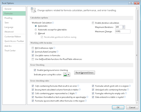
Figure 47-1:
Excel can check your formulas for potential errors.
When error checking is turned on, Excel continually checks your formulas. If a potential error is identified, Excel places an error indicator (a small triangle) in the upper-left corner of the cell. When the cell is activated, an error-checking button appears. Clicking this buttons provides you with a list of options. Figure 47-2 shows the options that appear when you click the error-checking button for a cell that contains a #DIV/0! error. The options vary, depending on the type of error.
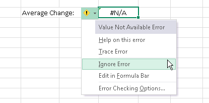
Figure 47-2:
Clicking an error-checking button gives you a list of options.
In many cases, you choose to ignore an error by choosing the Ignore Error option, which eliminates the cell from subsequent error checks. You can select a range of formulas, and then choose Ignore Error to ignore them all. All previously ignored errors can be reset so that they appear again. (Click the Reset Ignored Errors button in the Excel Options dialog box.)
Even if you don’t use the automatic error-checking option, you can choose the Formulas⇒Formula Auditing⇒Error Checking command to open a dialog box that displays each potential error cell in sequence, much like using a spell-checking feature. Figure 47-3 shows the Error Checking dialog box. Note that because it’s a modeless dialog box, you can still access your worksheet when the Error Checking dialog box is open.
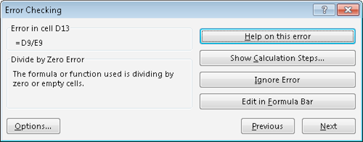
Figure 47-3:
Using the Error Checking dialog box to cycle through potential errors identified by Excel.
 Understand that the error-checking feature isn’t perfect. In fact, it’s not even close to perfect. In other words, you can’t assume that you have an error-free worksheet simply because Excel doesn’t identify any potential errors! Also, be aware that this error-checking feature doesn’t catch a common type of error — overwriting a formula cell with a value.
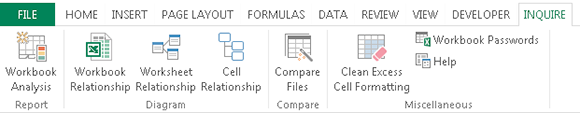
Tip 48: Using the Inquire Add-In
Office 2013 Professional Plus includes a handy auditing add-in called Inquire. To install this add-in, follow these steps:
1.
Choose File⇒Options to display the Excel Options dialog box.
2.
Click the Add-Ins tab.
3.
Choose COM Add-Ins from the Manage drop-down list and click Go to display the COM Add-Ins dialog box.
4.
In the COM Add-Ins dialog box, select the Inquire item and click OK.
If the Inquire item is not in the list, that means your version of Office doesn’t include this add-in.
When the Inquire Add-In is installed, Excel displays a new tab: Inquire (see Figure 48-1).