X and the City: Modeling Aspects of Urban Life (56 page)

This is also readily verified by direct substitution (exercise!). Generally,
K
₂
will also depend on the constants
D
and
U
. (We have simplified things greatly here; generally
D
will be different in the horizontal
y-
direction, perpendicular to the wind, from that in the vertical
z
-direction.) Note that, for a given distance
x
downstream, the maximum concentration is
C
(
x
, 0, 0) =
K
₂
(
D
,
U
)/
x
.

Now let’s think “laterally” for a moment; the right-hand side of equation (19.9) looks suspiciously like the equation of the
normal distribution
. (I have a now-defunct ten Deutschmark bill with the equation and graph of that distribution on it.) This has the classic “bell-curve” shape. In statistics, the random variable
X
is said to be normally distributed with mean
μ
and standard deviation
σ
if its probability distribution is given by

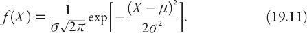
The total area between the
X
-axis and the graph of the function
f
(
X
) is equal to one (see
Figure 19.1
). If we compare equation (19.11) for
f
with that for
C
(
x
,
y
) above in equation (19.9), it is clear that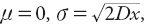
and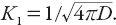
Carrying this equivalence over to the solution (19.10) for
C
(
x
,
y
,
z
), we see that the plume concentration is distributed normally in the crosswise direction (
y
) but also vertically (
z
), because now
and
The standard deviation
σ
is a measure of how tightly the concentration sits about the mean value
μ
(zero here); so the plume width in the
x
- and
z
-directions is here proportional to
, the square root of the distance downstream. It is also proportional to the square root of the diffusion coefficient and inversely proportional to the square root of the wind speed
U
. It is known that turbulence can increase
D
(which in this context is often referred to as the eddy diffusivity).

In light of these comments, let us summarize the predictions of the above model based on the solution (19.10) for
C
(
x
,
y
,
z
) now dropping the subscript on
K
₂
:

Figure 19.1. Normal distribution
f
(
X
) given by equation (19.11) for
μ
= 4 and
σ
= 4.

   I. The downwind concentration is directly proportional to
K
(
D
,
U
), the source emission rate.

  II. The more turbulent the atmosphere, the wider the lateral spread of the plume after any given time.

 III. The maximum concentration at any location is found at ground level on the line
y
= 0, and is inversely proportional to distance
x
downwind from the source.

A more general analysis of the particle emission problem shows that
K
∝
U
⁻¹
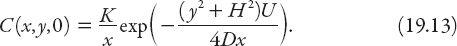
, so that the maximum concentration will be smaller for higher wind speeds. But even a less sophisticated model such as ours can be adapted to emission from an elevated source. A common example is the plume of smoke from a smokestack. Because the particles have a longer time to diffuse before they reach the ground, we expect that the maximum concentration will depend on the height
H
of the stack. Let’s investigate this. The simplest and most obvious modification to the model is to replace
z
by
z
−
H
in equation (19.10) for
C
(
x
,
y
,
z
). However; there is now a lower boundary for the particles—the ground—and the associated problem of what boundary condition to impose
on the problem. At this point the reader may object: in the previous model the source is on the ground at “height”
z
= 0; so why worry about the effect of ground in this model? In that case the maximum concentration was always at ground level, so the effect was implicit in the model. As we shall see, a simple modification is to assume that particles are partially reflected from the ground when they diffuse and settle downward. Perfect reflection is unlikely, of course; the ground is not a mirror and the particles are not perfectly elastic—indeed, recalling the difference that clay or grass courts can make in tennis, the problem is rather more complex than we can investigate in depth here. Nevertheless, some insight into the modeling process and the conclusions drawn from it can be illustrated by assuming that there is an “image” smokestack emitting pollutants at a rate
αK
(0 ≤
α
≤ 1) from
z
= −
H
. Of course, this is just a mathematical artifact (and a common one in this kind of problem). We are only interested in what happens for 0
z
≥ 0. To this end, the suggested form for the concentration distribution is

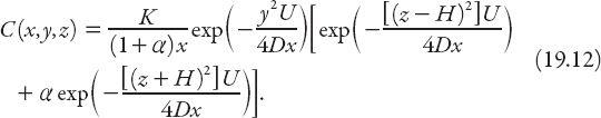
The divisor 1 +
α
in this expression is required to ensure that
C
reduces to the case above when
H
= 0. Again, we are interested in the concentration at ground level, which simplifies to