Understanding Sabermetrics (30 page)
Read Understanding Sabermetrics Online
Authors: Gabriel B. Costa,Michael R. Huber,John T. Saccoma

Figure 12.6. Scatterplot of OPS versus runs for the 2006 season
Fitting a trend line to the data gives encouraging results. In Figure 12.8, we again show the data with the trend line based on the least squares method. The equation of the line is
Runs = 2159.7 × OPS - 872.41
The coefficient of correlation is over 87 percent. This is a valid example of applying a linear regression to data using a single independent variable (OPS).
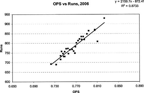
Figure 12.7 Scatterplot of OPS versus runs with trend line for the 2006 season
As mentioned earlier, we would like to apply this technique to more data. In Figure 13.8, we show a scatter plot of OPS versus runs scored for five seasons, 2002 through 2006. The data appears to exhibit a strong trend. The equation of the regression line is now
Runs = 2171.3 × OPS - 877.37
This equation is very similar to the one developed for just the 2006 data. In addition, the R
2
value has increased to 89.66 percent, or almost 90 percent.
2
value has increased to 89.66 percent, or almost 90 percent.
Next we try to model the runs-scored data with multiple variables. We will use a simple linear model, where we attempt to predict runs as a function of both on-base average (OBA) and slugging percentage (SLG), given by
Runs =
β
0
x OBA +
β
2
x SLG
Using just the 2006 data (30 data points), we find that the regression equation is given by Runs = - 924.30 + 2585.19 × OBA + 1948.31 × SLG, which yields a correlation coefficient of 87.78 percent, or almost half a percent better than using single-variable regression. Using all 150 data points from the 2002 through 2006 seasons, we develop a regression equation of Runs = - 948.02 + 2696.44 × OBA + 1925.21 × SLG, which yields a correlation coefficient of 90.00 percent, again slightly better than using single-variable regression. The coefficients for each independent variable do not change significantly when more data is added.
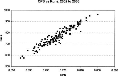
Figure 12.8 Scatterplot of OPS versus runs for the 2002 to 2006 seasons
We hope that we have provided an introduction into simulation and regression which will allow the reader to get started in analyzing baseball data. It is not a trivial process, but it can offer insights which might not be available using commonly-accepted sabermetrical measures.
Easy Tosses1. Create a simulation in which a batter has an equal chance of getting 2, 3, 4, or 5 at-bats in a game (assume that he will get only one of those outcomes). Use a batting average of .300 and simulate a 150-game season (our batter sits out a few games during the season). After the simulation, how does the simulated batting average compare to the input batting average?
2. Several studies have been done to predict runs scored using offensive measures such as RBIs, OPS, and batting average. Select thirty players with a similar number of at-bats from a given season and try to predict the runs scored.
Clubhouse: Answers to Problems
Before the 1990s, Pirate Hall of Famer Ralph Kiner had the second-best career home run percentage behind Babe Ruth (with Harmon Killebrew a tad behind Kiner). Ruth was the first player in history to hit 30, 40, 50 and 60 home runs in a season. Following 1961, and some years after, many people still argued that Ruth, not Roger Maris, held the seasonal home record, due to the extended 1961 season (162 games versus 154 games in Ruth’s time). Ruth held the season home run percentage mark as well.
Over the past ten years or so, however, sluggers like Sammy Sosa, Mark McGwire and Barry Bonds have surpassed many of Ruth’s accomplishments. Apart from the questions and controversies which have been raised, one fact seems to endure. No player in history has out-homered teams 90 times; or pairs of teams, which Ruth accomplished 18 times. It would seem that Ruth is still mighty and still prevails.
Inning 1: Simple Additive Formulas(1)
(2)
(3)
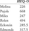
Sample calculation: Pujols: HEQ-O = TB + R + RBI + SB + 0.5 × BB = 359 + 119 + 137 + 7 + 0.5 × 92 = 668
(4)
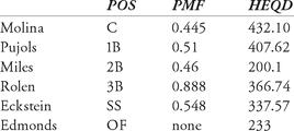
Sample calculation: Molina: HEQ-D = C: (PO + 3 A + 2 DP - 2 E) × (0.445) = (736 + 3(77) + 2(6) - 2(4)) × (0.445) = 432.095.
If Molina’s putouts were greater than 800, we would have assigned him 800 putouts.
(5)
(6)
Total Average = (TB + BB + HBP + SB) / (AB-H + SH + SF + CS + GIDP)
Pujols: (359 + 92 + 4 + 7) / (535 - 177 + 0 + 3 + 2 + 20) = 1.2063
Howard: (383 + 108 + 9 + 0) / (581 - 182 + 0 + 6 + 0 + 7) = 1.2136
Hard Sliders(1)
Thus, in 1966, the AL had a POP of .915 and Robinson’s was 1.363. Thus, his relative POP was 1.363 / 0.915 = 1.490 , meaning that Robinson’s POP was 49 percent better than the league average.
Other books
Flesh Collectors by Fred Rosen
Blind Descent-pigeion 6 by Nevada Barr
Overkill by Castillo, Linda
Aelred's Sin by Lawrence Scott
A Field of Red by Greg Enslen
Jonathan Livingston Seagull: The New Complete Edition by Richard Bach, Russell Munson
Uncharted (Treasure Hunter Security Book 2) by Anna Hackett
The Chessman by Jeffrey B. Burton
Glass Towers, Shattered (Glass Towers Trilogy) by Adler, Holt


