Understanding Sabermetrics (27 page)
Read Understanding Sabermetrics Online
Authors: Gabriel B. Costa,Michael R. Huber,John T. Saccoma

Extra Innings: Beyond Sabermetrics
Those who practice sabermetrics are searching for objective truth in baseball. They try to determine who the best players were (and are), by developing formulae that compare and contrast players. They have looked at the simple statistics of the first 100 years of major league baseball and tried to create well-accepted measures, starting with batting average and earned run average, and then moving to runs created, linear weights, and win shares, to support their claims. Can we develop predictions and rankings of players and teams with sabermetrical analyses alone? Several major league baseball teams are now using full-time professional statistical analysts to find patterns to provide valuable information to managers. Managers then can decide whether to use this statistical information in making decisions during a game. There are a host of sabermetrical websites, including
mlb.com
, which provide data and trends directly to the ballclubs. Baseball statisticians have popularized the notion that it is possible to answer a variety of questions about the game by means of statistical analyses. In this chapter we go beyond the accepted stats and ponder more rigorous statistical analyses. We will develop the ideas behind simulation and regression, useful tools in developing measures to analyze complicated data.
Simulationmlb.com
, which provide data and trends directly to the ballclubs. Baseball statisticians have popularized the notion that it is possible to answer a variety of questions about the game by means of statistical analyses. In this chapter we go beyond the accepted stats and ponder more rigorous statistical analyses. We will develop the ideas behind simulation and regression, useful tools in developing measures to analyze complicated data.
As a first example, let’s consider that in 1941, Joe DiMaggio was 26 years old and already a star on the New York Yankees. The Yankees had won the World Series in each of DiMaggio’s first four seasons, 1936 through 1939, but were coming off of a third-place finish in 1940. DiMaggio had won the Most Valuable Player Award in 1939, and he had finished third in the MVP voting in 1940, behind Hank Greenberg and Bob Feller. He had been named to the American League All-Star Team in each of his first five seasons. In 1940, DiMaggio was the club leader in batting average, on-base percentage, slugging percentage (and therefore in OPS), hits, total bases, home runs, runs batted in, singles, adjusted OPS+, runs created, at-bats per strikeout, and at-bats per home run. It was good to be Joltin’ Joe DiMaggio, the Yankee Clipper. Could it get any better?
As you already know, 1941 became the year that Joe DiMaggio established the one record that will probably never be broken. He hit safely in 56 consecutive games, breaking Wee Willie Keeler’s mark of 44 straight games, set in 1897. DiMaggio became only the third player in the twentieth century to hit safely in at least 40 consecutive games (the others being Ty Cobb with 40 in 1911, and George Sisler with 41 in 1922) Pete Rose in 1978 would become the only other player to hit in at least 40 straight games.
Never be broken, you ask? How can we be sure? Let’s go beyond the sabermetrics and create a simulation of Joe DiMaggio’s 1941 season. Several researchers have investigated DiMaggio’s hitting streak, creating complicated simulations and resolving probabilities in a game-to-game fashion. We seek to simulate a hitting streak in a simple yet reliable manner. Let’s develop the tools necessary to recreate the opportunity that Joe had. First, in order to create an effective simulation, we look at the actual data from 1941.
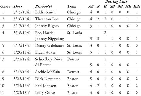
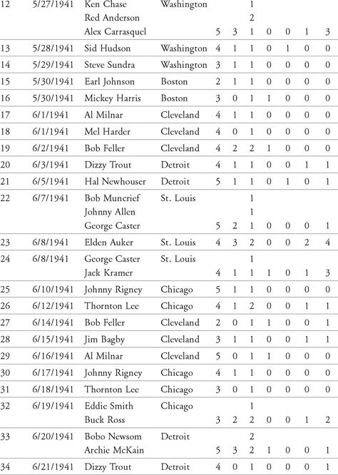
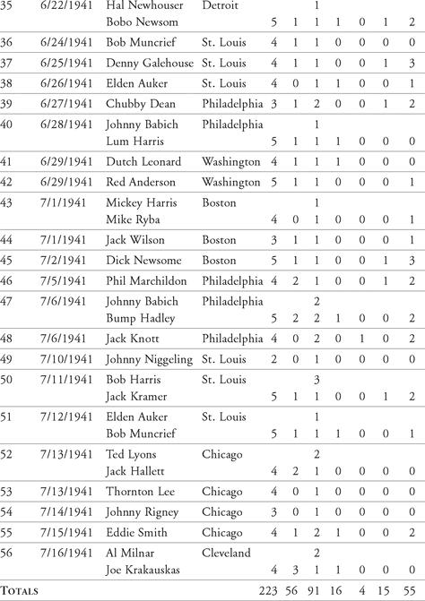
From this data, we’ll develop a table of outcomes from the hitting streak. For example, we notice that Joe had at least two at-bats in every game of the streak. The most at-bats in a single game was five. Therefore, we create a table showing the distribution of at-bats in the 56 games. Table 12.1 shows this distribution. In the first column are the number of possible at-bats. In the next column are the observed values for each amount of at-bats. Next is the percentage of that number of at-bats occurring (the count divided by 56, the total number of games in the streak). The last column shows the cumulative percentage for up to six at-bats in a single game.
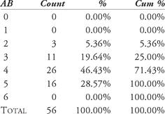
Table 12.1 Distribution of at-bat occurrences
Table 12.1 shows us that Joe had 11 out of 56 games in which he had three official at-bats, or he had three at-bats in 19.64 percent of the games during the streak. Further, he had
no more than
three at-bats in 25 percent of the 56 games. In a simulation of the streak, we would expect him to have similar percentages of games with three or fewer at-bats. We note a few things here. Is it possible to have no at-bats, or just one at-bat in a game? Rule 10.24 of the
Major League Baseball Official Rule Book
provides the following guidelines for cumulative hitting streaks:
First, “a consecutive hitting streak shall not be terminated if the plate appearance results in a base on balls, hit batsman, defensive interference or a sacrifice bunt. A sacrifice fly shall terminate the streak.” This means that if Joe had no official at-bats in a game (for example, he walked in four plate appearances), the streak would continue.
Second, “a consecutive game hitting streak shall not be terminated if all the player’s plate appearances (one or more) result in a base on balls, hit batsman, defensive interference or a sacrifice bunt. The streak shall terminate if the player has a sacrifice fly and no hit. The player’s individual consecutive game hitting streak shall be determined by the consecutive games in which the player appears and is not determined by his club’s games.” This is very similar to the first guideline from the
Official Rule Book
, except it points out that a hitting streak remains intact if the player sits out a game, even though the team plays.
Official Rule Book
, except it points out that a hitting streak remains intact if the player sits out a game, even though the team plays.
How does this affect the probabilities? The probability of getting no at-bats during a hitting streak is zero. Even though Joe had no games with only one at-bat, the probability exists that it could occur, so in the simulation, we will designate a probability (albeit a small one); we fix the probability of one at-bat in a game to be 0.10 percent. Similarly, although Joe did not have any six-at-bat games, we will fix the probability at 0.10 percent that it could occur. We will not expect any single games with at-bats greater than six. Table 12.2 shows the adjusted table of probabilities. The last column is just a decimal representation of the percentage.
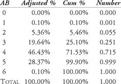
Table 12.2 Distribution of adjusted at-bat percentages
Now we are ready to begin the simulation. Using a spreadsheet program (such as Microsoft Excel), we will generate random numbers. We need to determine the number of official at-bats per game and then determine whether or not each at-bat results in a hit or in an out. Take a look at Figure 12.1. This shows a screen capture of one such simulation.
In the upper left we designate a batting average (shown in cell D2) of 0.333. Our screen capture has a “slider bar” to adjust the batting average, but that is not necessary. This simulation will model a 162-game season. Column B in the spreadsheet shows the game number. In column C, we generate a random number, which will determine the number of at-bats in the game. For example, the computer generated 0.233 (cell C8 in Figure 13.1). Looking at the right-most column of Table 13.2, we see that 0.233 falls between 0.055 and 0.251 (the chance of 2 and 3 at-bats). Therefore, we set the at-bat value at 3 (see cell D8), using a conditional formatting command. Since the random number generated in cell C9 is 0.357 (between 0.251 and 0.715), the number of at-bats is 4 (cell D9). This process is repeated for all 162 games. Next we generate six random numbers for each possible at-bat (columns E through J). The output of each number will be displayed in columns K through P. Depending on the value of cell D8, only those columns corresponding to the number of at-bats are used. The computer compares the random number generator to the batting average. If the random number is less than or equal to the batting average, we record “Hit”; otherwise, we record “Out.” Notice in Figure 12.1 that the first hit occurs in the fourth game. Cell H11 has a random number of 0.130, which is less than 0.333. You may have noticed that cell H8 also has a value lower than 0.333; however, Game 1 only had three at-bats, so this number is not used. Continue this process for all 162 games. As an added feature, we count the number of hits in a game in column Q. In Game 4 (row 11 of the spreadsheet), the batter broke out of the slump, going 1 for 5. In Game 26 (row 33) he went 4 for 5. Column R counts the number of consecutive games with a hit. Using an “IF” statement, we add up the number of games with hits. If the value in column Q is a number other than 0, we add one to the previous value in column R. So, returning to game 4, the value in cell Q11 is a 1. The value in R10 is a 0, so we add 1 to it, creating a 1 in R11. The batter also got a hit in game 5, so the value in cell R12 is 1 + 1 = 2. Notice that from game 20 through game 40, our batter with a 0.333 batting average had a 21-game hitting streak. The maximum streak for a 162-game season can also be displayed at the top of the spreadsheet (cell K2). Finally, we can add up all of the at-bats in the simulation (in this simulation we had 642 at-bats). In addition we can add up the total number of hits (228) and determine that the batter had a seasonal batting average of .355 (shown in cell G4).
Other books
Until Dark by Mariah Stewart
Galatea by James M. Cain
Fair Game by Malek, Doreen Owens
The Dog House (Harding's World of Romance) by Harding, Nell
Scorching Desire by Lila Dubois, Mari Carr
How to Seduce a Vampire (Without Really Trying) (Love at Stake) by Kerrelyn Sparks
Dark Side of the Laird (Highland Bound) by Knight, Eliza
Missing by Sharon Sala