Nonplussed! (18 page)

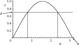
Figure 7.6.
The experiment’s phase space

and so arrive at the remarkable fact that

and hence at an experimental method of approximating
π
.

If we revert to the empirical, for a given length of needle and distance between parallel lines, we can perform the experiment repeatedly in the manner of our Victorian forbears (or get a computer random number generator to do the work for us) to compute the value
C
/
R
.

In fact, ‘throwing the needle’ 10 000 times with
l
= 1 and
d
= 2 led to the result

which, of course, means that
π
≈ 3.143 17 ….

Buffon’s (Long) Needle

The condition that
ensures that
l
sin
and therefore that the curve lies within the rectangle in
figure 7.6
. If we wish to conduct the experiment with
l
>
d
,
l
sin
θ
may well be greater than
d
and we will need to take into account the overlap of the curve and the rectangle, as shown in
figure 7.7
, and compute the area under the truncated curve.

Figure 7.7.
The modified phase space

The intersections are where
l
sin
θ
=
d
, or = sin
⁻¹
(
d
/
l
), and
π
− sin
⁻¹
(
d
/
l
). The area we want is then

where the cos(sin
⁻¹
(
d
/
l
)) is transformed to the more convenient
by use of the standard mechanism that if
θ
= sin
⁻¹
(
d
/
l
), sin
θ
=
d
/
l
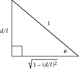
and so the triangle shown in
figure 7.8
exists and the third side is found by using Pythagoras’s Theorem, which makes cos

And all of this makes the probability of a crossing at least one line the rather more impressive expression

Figure 7.8.

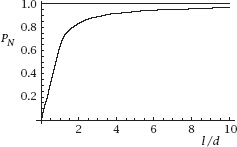
Figure 7.9.
The full story

To summarize, the probability,
P
_N
, of the needle crossing at least one line is given by

Notice that, not unreasonably, the two formulae agree at
l
=
d
.
figure 7.9
is a plot of this combined probability function against
l
/
d
.

The Lazzarini Entry